background

after built the Gitlab server in LAN for two month, managing about 20 projects in ADS group currently. the needs for CI is coming up. at very beginning, I tried Gitlab CI runner, doesn’t work through. so Jenkins!

Jenkins installation

there is a great series Maxfields jekins-docker tutorial, since originally I had Docker env and which is a prepartion for cloud deployment in future.

• Jenkins in Docker installation,

• start Jenkins in Docker

1

docker run --rm -p 8080:8080 -p 50000:50000 -v jenkins-data:/var/jenkins_home -v /var/run/docker.sock:/var/run/docker.sock  jenkinsci/blueocean

• setup wizard

also Jenkins installed directly in Ubuntu

Jenkins integrated with Gitlab

Jenkins default has integrated with BitBucket and Github, to integrate with Gitlab:

• set Gitlab token

in Gitlab Project main page, go to User Profile >> Settings >> Peronsal Access Token, naming the token and click api domain, the token is generated.

• install Gitlab Plugins

in Jenkins main page: Manage Jenkins >> Manage Plugins >> Search Available Plugins (gitlab).

• add gitlab key credentials

in Jenkins main page, go to Credentials, choose the key type to Gitlab API token, then generate the key credential, used to access Gitlab project.

• configure Jenkins with gitlab

in Jenkins main page, go to Manage Jenkins >> Configure System, at the gitlab section, add the gitlab host url and use the credential created at previous step.

since the gitlab server is hosted in LAN, even don’t have DNS for the gitlab server, purely raw IP address. so the gitlab host URL is like:

http://10.20.110.110:80 

rather than the project git url (e.g. http://10.20.110.110/your_name/your_project.git)

Gitlab Hook Plugin

gitlab events will be post to Jenkins through webhook, which is a common way to notify external serivces, e.g. dingding office chat, JIRA e.t.c. To set it up, need to configure Gitlab Hook plugin in Jenkins.

as mentioned in this post, JDK10 or 11 is not supported for Jenkins, if the current OS system has already JDK11, need addtionally install jdk8, and configure the default jdk=8:

1
2
3
4
5
6

update-java-alternatives --list 
sudo update-alternatives --config java 
java -version

Jenkins Project

add a new Jenkins Item, select FreeStyle, go to Configure.

in Source Code Management section, select Git. add Repository URL and set gitlab username and password as Jenkins Credentials.

in Build Triggers section, select Build when a change is pushed to Gitlab, which display the Gitlab webhook URL: http://localhost:8080/jenkins/project/demo; go to Adavance section to generate the secret token.

when getting all these done, back to Gitlab project, as Admin or Maintainer, in Project Settings >> Integrations >> Add Webhooks.URL and Secret Token are from the previous settings.

there is a common issue: Url is blocked: Requests to localhost are not allowed, please refer to allow request to localhost network from system hooks

refer

riot games: putting jenkins in docker

jenkins to gitlab authentication

devops expert: Emil

mind the product: PM’s guide to CD & DevOps
manage multi version of JDK on Ubuntu

a jianshu refer

a aliyun refer

tencent refer

allow request to localhost network from system hooks

abstract space

• Cauchy Series

in metric space, existing an any positive and small \etta, exist a natural number N, $m, n > N$, which satisfies:

it’s called a Cauchy Series. intuitively, as the numbers goes above, the elements get closer.

• Complete Space

any Caunchy Series in these abstract space, its convergence is still in the original space.

e.g. rational number space is not complete space, as is not in rational number space anymore.

intuitively, a complete space is like a shell without any holes on its surface.

• Linear Space

with linear structural set, which can be described by base vector, so any hyper-point in a linear space can be represented by the linear combination of its base, so also called as vector space. in another way, linear space has only add and scalar multi operator.

• Metric Space

to describe length or distance in linear space, adding normal in the linear space, gives normed linear space or metric space.

• Banach Space

a complete metric space

• Inner Product Space

with inner product feature in metric space. for the infinite space, there are two different sub space, either the inner product of the series converged or not.

the convergence sub space is a completed space.

• Hilbert Space

a completed inner product space

• Eurepean Space

a finite Hilbert Space.

functional analysis

the optimzed control theory problem, is to find the functional, under system dynamic constraints, which gives the extremum point(function) in the infinite normed linear space; in general.

in general, the functional is depends on the system dynamic path, which gives some famuous theorem: Banach fixed point.

PDE theory, partial geometry, optimized control theory are all part of functional analysis. from computational mechanics field, there is a chance go to PDE theory; from modern control field, there is a chance go to optimized control theory; from modern physics field, the students may also get familiar with partial geometry. the beauty of math is show up, all these big concepts finally arrive to one source: functional analysis.

to transfer all these big things into numerial world, which gives CAE solver, DQN solvers e.t.c.

the closest point property of Hilbert Space

A subset of A of a vector space is convex: if for all a, b belongs to A, all \lamba such that 0 < \lamba < 1, the point belongs to A

assuming A is non-empty closed convex set in Hilbert Space H, for any x belongs to H, there is a unique point y of A which is closer to x than any ohter point of A:

orthogonal expansions

if (e_n) is an orthonormal sequence in a Hilbert space H, for any x belongs to H, (x, e_n) is the nth Fourier coefficient of x with respect to (e_n), the Fourier series of x with respect to the sequence (e_n) is the series:

• pointwise converges

where f_nis a sequence of functions in

• complete orthonormal sequence

given an orthonormal sequence of (e_n) and a vector x belongs to H then:

but only when this sequence is complete, the right-hand side converge to left-hand side workks.

an orthonormal sequence (e_n) in Hilbert Space H is complete if the only member of H which is orthogonal to every e_n is the zero vector.

a complete orthonal sequence in H is also called an orthonormal basis of H.

H is separable if it contains a complete orthonormal sequence,

the orthogonal complement (which named as E^T) of a subset E of H is the set:

for any set E in H, E^T is a closed linear subspace of H.

the knowledge above gives the convergence in Hilbert Space, application like FEA, once created the orthonormal basis of solution space, the solution function represented by the linear combination of these basis is guranted to convergence.

Fourier series

it is a complete orthonormal sequence in L^2(-\pi, \pi), and any function represented by a linear combination of Fourier basis is converged.

but here Fourier basis is the arithmetic means of the nth partial sum of the Fourier series of f, not the direct basis itself.

Dual space

FEA solutions for PDE

PDE can be represented in a differential representation:

or an integral representation:

integral formulation has included existing boundary conditions. by multiplying test function \phi on both side of integral representation, and using Green’s first identity will give the weak formulation(variational formulation) of this PDE.

in FEA, assuming the test function \phi and solution T belong to same Hilbert space, the advantage of Hilbert space, is functions inside can do linear combination, like vectors in a vector space. FEA also provides the error estimates, or bounds for the error.

the weak formulation should be obtained by all test functions in Hilbert space. this is weak formulation due to now it doesn’t exactly requries all points in the domain need meet the differential representation of the PDE, but in a integral sense. so even a discontinuity of first derivative of solution T still works by weak formulation.

Hilbert space and weak convergence

convergence in another words means, the existence of solution. for CAE, DQN algorithms, the solution space is in Hilbert space.

Lagrange and its duality

to transfer a general convex optimization problem with lagrange mulitplier:

=>

we always looks for meaning solution, so L should exist maximum extremum. if not, as x grow, the system goes divergence, no meaningful solution. define:

so the constrainted system equation equals to :

to rewrite the original equation as:

then the system’s duality is defined as :

for a system, if the original state equation and its duality equation both exist extremum solution, then :

the benefits of duality problems is

• the duality problem is always convex, even when the original problem is non-convex

• the duality solution give an lower boundary for the original solution

• when strong duality satisfy, the duality solution is the original solution

Krylov Space

refer

convex func

finite element method

Lagranget duality

standford convex optimization

Going deeper into RF: understaing Q-learning and linear function approximation

Nicholas Young, an introduction to Hilbert Space

why are Hilbert Space important to finite element analysis

RL concepts

assuming timestep t:

• the environment state S(t)
• agent’s action A(t)
• discouted future reward R(t), which satisfy:

with current state `s` and taking current action `a`, the env will give the reward `r_{t+1}`. `\gamma` is the discount ratio, which usually in [0,1], when $\gamma = 0 $, agent's value only consider current reward.  check [discount future reward]() in following chapter.

• agent’s policy P(a|s), in current state s, the propability of action a

• agent’s state value V(s), in state s and took policy \pi, which usually described as an expectation:

• agent’s action value Q(s, a), which consider both state s and action a effects on value calculation.

namely, agent’s value is the expectation of its action value with probability distribution p(a|s).

• state transfer propability P
• explore rate \eta, it’s the chance to choose non-max value during iteration, similar as mutation.

Markov decision process

assuming state transfer propability, agent's policy, and agent's value follow Markov assumption. namely, the current state transfer propability, agent’s policy and value only relates to current state.

agent’s value function V(s) meets Belman’s equation:

and agent’s action value function q(s) also has Belman’s equation:

in general, env’s state is random; the policy to take action is policy P(a|s). Markov Decision process is: state, action, policy, each [state, action, policy] is an episode, which gives the state-action-reward series:

s0, a0, r1, s1, a1, r2, ... s(n-1),  a(n-1), rn, sn

Markov assumption is state(n+1) is only depends on state(n).

Belman’s equation

Belman’s equation gives the recurrence relation in two timesteps. the current state value is calcualted from next future status with given current env status.

discounted future reward

to achieve better reward in long term, always conside the reward as sum of current and future rewards:

R(t) = r(t) + r(t+1) + ... r(n)

on the other side, as the env state is random in time, the same action doesn’t give the same reward usually, and as time goes, the difference is even larger. think about the B-tree, as it goes deeper, the number of nodes is larger. so the reward in future doesn’t count the same weight as earlier reward, here define the discount ratio \gamma <- [0, 1]

R(t) = r(t) + \gamma r(t+1) + ... + \gamma^(n-t) r(n)

R(t) = r(t) = \gamma R(t+1) 

policy iteration

there are two steps:

• policy evaluation, with current policy \pi to evaluate state’s value V'

• policy improvment, with the state value V', with a special policy update strategy(e.g. greedy) to update policy.

the ideal result is to find the fixed point in value space, which corresponds to the optimized policy at current state with current policy update strategy.

in policy iteration, we only consider policy-value mapping.

value iteration

where policy iteration based valued is implicit, only value iteration explicit by Belman’s equation. this is also a fixed point application, as we can use the explicit mapping (Belman’s equation) in state value space. so there should guarantee existing an optimized policy.

an optimization problem

reiforcement learning solution is to find the optimal value function to achieve the max reward in each timestep, which leads to optimal policy \pi*, or max value func, or max action value func.

$$ v(s) = max(v_i(s)) foreach i in value funcs $$ 

$$ q(s, a) = max(q_i(s,a)) foreach i in action value funcs $$ 

mostly the solution space is not known at hand, if else, the optimal solution can get directly. on the other hand, current state, action set tells a little information about the solution space, as they are part of the solution space, so the optimization algorithms used in convex space can be applied here.

a few common optimization algorithms includes:

dynamic programming(DP)

DP can used in both policy evaluation and policy iteration, but in each calculation step(not even one physical step, and in one physical step, there can be hundreds or thousands of calculation steps) iteration, DP has to recalculate all state(t=current) value to the very first state(t=0) value, which is disaster for high-dimensional problem, and DP by default is kind of integer programming, not fitted to continuous domain either.

Monte Carlo (MC)

MC gets a few sample solutions in the solution space, and use these samples solution to approxiamte the solution space. in a geometry explaination, the base vectors of the solution space is unknown, but MC finds a few points in this space, then approximate the (nearly) base vectors, then any point in this space can be approximated by the linear combination of the nearly base vectors.

MC has no ideas of the propability of state transfer, MC doesn’t care the inner relations of state variables, or model-free.

MC is robost as it’s model free, on the other hand, if the solution space is high-dimensional, there is a high chance the sampling points are limited in a lower dimension, which weak the presentation of MC approximation; also MC needs to reach the final status, which may be not avaiable in some applications.

time-serial Time Difference(TD)

MC use the whole list of status for each policy evaluation; in 1st order TD, policy evaluation only use next reward and next state value:

$ v(s) = R(t+1)  + \gamma S(t+1)|S $

for n-th order TD, the update will use n-th reward :

$ v(s) = R(t+1) + \gamma R(t+2) + ... + \gamma^(n-1) R(t+n) + \gamma^n S(t+n)|S $

it’s clear here, as n->infinitly, n-th order TD is closer to MC. so how close is enough usually, namely which n is enough ?

SARSA

in TD, there are two ways: on-line policy, where the same one policy is using to both update value func and upate action; while off-line policy, where one policy is used to update value func, the other policy is used to update action.

SARSA is kind of on-line policy, and the policy is e-greedy, to choose the max value corresponding action in every iteration with a high probablitiy (1-e), as e is very small.

$ \delta(t) v(S, A) = R + \gamma (v(S', A') - v(S, A)) $

in the iteration equation above, \delta(t) will give the iteration timestep size, S', A' are next state and next action, compare to pure 1-st order TD, where the next state value is modified as: $(Q(S’, A’) - Q(S, A)$, in this way value func keep updated in every func, which can be considered as local correction, compared to the unchanged pure 1-st order TD, which may be highly unstable/diverge in long time series.

as time-serial TD can’t guarantee converge, so this local correction makes SARSA numerical robost.

SARSA(\lambda) in mutli-step based is same as n-th order TD.

$ v(s) = R(t+1) + \gamma R(t+2) + ... + \gamma^(n-1) R(t+n) + \gamma^n ( v(S`) - v(S) ) $

the problem of SARSA is v(S, A) may go huge, as the algorithm is on-line policy, which requires huge memory.

Q-learning

Q-learning is off-line policy TD. the policy iteration is use e-greedy policy, same as SARSA; while the policy evaluation to update value func use greedy policy.

in a word: from status S, using e-greedy policy to choose action A, and get reward R, and in status S', and using greed policy to get action A'.

$ \delta(t) Q(S, A) = R + \gamma (Q(S', A') - Q(S, A)) $   (a)

where $ A= max v(a|S) $. while in SARSA, both S' and A' update using e-greed.

usually Q(S,A) is called Q-valued.

the benefit of choosing a different policy to update action, is kind of decouping status and action, so in this way, they can reach more area in real state-action space, which also lead the solution space a little more robost.

but still equation (a) is not guaranted to converge as time goes. the converged Q(S,A) should be convex, which means its second-order derivative must be less than 0, then the max Q values (max extremum) achieves when first-order derivate is 0.

while Q-learning has the same problem as SARSA, the huge memory to store Q(S,A) table.

to make intuitive example, think about an robot walk with 2 choice(e.g. turn left, turn right), and the grid world has 20 box in line, which has 2^20 ~= 10e6 elements in Q(S, A). it can’t scale to any real problem.

refer

Sutton & Barto, Reinforcement learning: an introduction

Pinard

fromeast

mathxml editor

equation html editor

fixed point mechanism

unittest

why unit test ?

unit test is to test the components of a program automatically. a few good reasons of unit tests:

• test driving practice
• early sanity checking
• for regression test, that the new changes won’t break early work
• unit test is to test the isolated piece of code, usually white box test written by developer; functional test is to test the function requirements, usually black box test written by testers.

the testcase output can be OK, FAIL, ERROR.

assertion functions

• basic boolean asserts:

  assertEqual(arg1, arg2, msg=None)
  assertIsNot(arg1, arg2, msg=None)
  

• comparative asserts:

  assertAlmostEqual(first, second, places=7, msg=None, delta=None)
  

• asserts for collections:

  assertListEqual(list1, list2, msg=None)
  assertTupleEqual(tuple1, tuple2, msg=None)
  assertSetEqual(set1, set2, msg=None)
  assertDictEqual(dic1, dic2, msg=None)    
  

  command line interface

• run all unittests

  python3 -m unittest discover -v -c
  

• run single test module

  python3 -m unittest -v -c tests/test_XXXX.py
  

• run individual test case

  python3 -m unittest -v tests.test_XXX.TestCaseXXX.test_XXX
  

how to write a unittest

unittest.TestCase

any user defined test class should first derived from unittest.TestCase

setUp() & tearDown()

setUp() provides the way to set up things before running any method starting with test_xx() in user defined test class. tearDown() is where to end the setting ups

depends on other modules/class

usually the class/methods we try to test have depends on other modules/class, but as unit test want to isolate these depends, so either mock the other methods or fake data. in general there are three types of depends:

pure variable

this is the most simple case, then you can directly define the same pure type variable in your test_xx() method

methods in other modules

here need to use patch, to mock the method and define its return value is your test_xx() method, then in the class where call the real method will be replace by this mocked one.

methods in other class

here need to use mock, either MagicMock or Mock will works.

mock & patch

mock module is built in unittest.mock after a later Python version, if not, mock module can be installed by pip install mock, then directly import mock in code.

the philosophy of unit test is to isolate classes test, but in reality most classes have some instances of other classes, so to test the ego class isolated from other classes, that’s where mock helps.

1
2
3
4
5
6
7
8
9
10
11
12
13
14
15

from mock import MagicMock, patch
class TestScenario(TestCase):
	
	def test_mock(self):
		sim.method = MagicMock(return_value="xx")
		agent = sim.method()
		self.assertEqual(agent, "xx")
		
	@patch("module/add_agent")
	def test_patch(self, mock_add_agent):
		mock_add_agent.return_value = "xx"
		agent = module.add_agent()
		self.assertEqual(agent, "xx")

Mock helps to mock the method in a class, while patch helps to mock a global method in a module.

automatical unittest generator

there are projects assit to generate unittest code automatically, e.g auger

test with while Loop

TODO

test with raise Error

TODO

coverage.py

• (one time only) install coverage.py

  pip3 install –user coverage

• run all tests with coverage

  ~/.local/bin/coverage run -m unittest discover

• generate html report

  ~/.local/bin/coverage html –omit “~/.local/“,”tests/“

ps, output is in htmlcov/index.html

logging

logging() supports more detail message type(info, warn, error, debug) than print(), and the message format is more strict with \%. while print() works both formatted message and message as string simply:

1
2

print("1+1 = ", num)
print("1+1 = %d", % num)

the following is a general log class, which can plug in any existing Python project:

import logging 
import os 

class log(object):
    def __init__(self, logger_name):
        self.log = logging.getLogger(logger_name)
        self.log.setLevel(logging.DEBUG)
        console_handler = logging.StreamHandler()
        console_handler.setLevel(logging.DEBUG)
        self.log.addHandler(console_handler)

    def set_output_file(self, filename):
        file_handler = logging.FileHandler(filename)
        file_handler.setLevel(logging.INFO)
        formatter = logging.Formatter('%(asctime)s - %(name)s - %(levelname)s - %(message)s')
        file_handler.setFormatter(formatter)
        self.log.addHandler(file_handler)

def main():
    test = log('scenario-mm')
    file_name = "record.log" 
    dir_name = "/home/python_test/"
    try:
        os.makedirs(dir_name)
    except OSError:
        pass 
    file_path =  os.path.join(dir_name, file_name)
    test.set_output_file(file_path)
    test.log.debug("debug in episode 1...")
    test.log.info("info ...")
    test.log.warning("warn ...")
    test2 = log("zjjj")
    test2.set_output_file('record.log')
    test2.log.info("test2 info")
    test2.log.warning("test2 warn")


if __name__ == "__main__":
    main()

pygame

refer

python automatic test series

auger: automated Unittest generation for Python

unittest official

unittest in lg-sim project

coverage.py official

unittest + mock + tox

when dealing with plan and control models in ADS system, there are plenty of basic math, and the understanding of these math are definitely helpful to build a better and stronger algorithm.

to design a ADS software system, there are two parts, the engineering background and software development. enginneering side is the core logic, while software is about how to organize the software and present, especially with new ideas, e.g. cloud based architecture, web user interface.

vector analysis

coordinate system

asssumed a Cartesian system [O: e1, e2, e3], a vector r can be represented as (x, y, z).

vector operator

• vector add

  a + b = (a_x + b_x) i + (a_y + b_y) j + (a_z + b_z) k

the triangle inequality is:

|a + b| <= |a| + |b|

• multiply scalar

  a . b = a . b_x i + a . b_y j + a . b_z k

namely, by multiplying each direction component of the vector by a.

• dot product

  a . b = |a|.|b|. \cos = a_x . b_x + a_y . b_y + a_z . b_z

a simple physical explaination: assume a is displacement, b is force, then the power of force in the displacement is by dot product.

the geometric meaning of dot product is projection. namely, |a|cos means project of vector a on vector b, which also gives the decomposion of a, which has a unique projection component vector and vertical component vector.

a = a_p + a_v

a_p = ( a . e_p ) . e_p

• cross product

assume three vectors non-co-plane, (a, b, c), rotating start from a to b, the thumb point to c, which is a right-hand-coordinate system.

a simple physical meaning: assume a is the force, b is the force arm, then a x b gives the torque, which perpendicular to plane.

a x b = |a||b| \sin

the geometric meaning of cross product is the area of parallelogram by .

base vectors in right-hand Cartesian coordiante system satisfy:

ei x ej = ek (i != j)

• mixed product

  $$ a x b \cdot c  $$
  

which gives the volume of parallel hexagonal propped by

curve(volume) integration

• Gauss integration

• Stokes integration

scalar field

• directional derivative

assuming vector l in space, its unitfied vector can be present as directional cosine [cos\alpha, cos\beta, cos\gamma]^T. for any function u=u(x, y, z), who is derivable at M0(x0, y0, z0), then:

\frac{\partial u}{\partial l} = dot_product(\Delta u, <\cos \alpha, \cos \beta, \cos \gamme> )

• gradient

  \Delta u =  \frac{\partial u}{\parial x} \b{i} + \frac{\partial u}{\parial y} \b{j} +  \frac{\partial u}{\parial z} \b{k}
  

the directional derivative which gives the maximum of \Delta u at a point, it’s the gradient direction. the gradient direction in space, stands for the direction from lowest co-value layer to highest co-value layer, which in physical, means the most high rate of change in general.

• Halmilton operator

  \Delta  =  \frac{\partial}{\parial x} \b{i} + \frac{\partial}{\parial y} \b{j} +  \frac{\partial}{\parial z} \b{k}
  

vector field

• directional derivative

the gradient field of a vector field gives a tensor field, which raise the dimension one more. the dot product(inner product) of a vector field, decrease to scalar field, the cross product of a vector field keeps a vector field. for a vector field, usually talk about its flux and divergence.

analytical geometry

plane equation

assume plane \pi in Cartesian coordinate system [O: X, Y, Z], O‘s projection in plane is N, the directional cosine of ON is (l, m, n),

for any point P in plane, NP is always perpendicular to the directional cosine, namely:

dot_product( NP, (l, m, n) ) = 0

as l**2 + m**2 + n**2 == 1, which gives:

lx + my + nz - p = 0            (1)

equation 1) is the normalized plane equation. and (l, m, n) is the normal vector of lane \pi, and p should be no lesss than 0.

linear equation

assumed a line go across point P_0 $(x_0, y_0, z_0)$ and in direction \lamba, then any point P $(x,y,z)$ on this line, satisfy:

x - x_0 = |PP_0| . l 
y - y_0 = |PP_0| . m 
z - z_0 = |PP_0| . n 

taking |PP_0| as t, the equation above is the parmeterized line equation, namely:

\frac{x-x0}{l} =  \frac{y-y0}{m} =  \frac{z-z0}{n} 

in general, a linear is the cross interface of two linear plane, so its genearl equation is to satisfy both plane equation:

A1.x + B1.y + C1.z + P1 = 0
A2.x + B2.y + C2.z + P2 = 0

coordiante transfer

in general, coordiante transfer means base vector linear transfer. assuming original coordinate system [O: e1, e2, e3], and new coordinate system [O’, e1’, e2’, e3’]

both the original base vector and new base vector <e1’, e2’, e3’> prop up the same 3D linear space.

and there should be transfer matrix between them:

e = matrix[3x3] \cdot e’

for any point P transfer from original to new coordinate system,

{x} = {a} + {x’} . matrix[3x3]

matrix[3x3] is:

each raw in the matix above, stands for a base vector tranfer from original one to the new one, namely:

$$ e1' = a11.e1 + a21.e2 + a31.e3 $$ 

the component value of each coordinate, can be simply by:

x1’ = e1’ . OP’

refer

write mathematic fomulars in Markdown

个人与公司的生存和发展法则。因为企业生存状态以及老板的眼光，国内企业会有一种氛围：老板花钱是让来工作的，来学习都不该提倡。个人而言，学习才能保持议价权。也需要有个良好的心态，面对这样的企业现状。

国内就业大环境也长期不看好。本来优质的大公司和岗位不多，相对缺乏壁垒的，最近的一个新闻： 一汽大众不招传统专业，比如，车辆、机械。不过话说回来，一汽大众的工作在长春也是绝对高薪。不招人背后，是技术岗位都在德国，那国内的年轻人在这样的企业怎么积累？ 当然，即使在这样的企业内，还会分三六九等。年轻人被局限的穷迫程度可想而知，这样缺乏格局的环境，也没办法培养年轻人的领导力。

上一篇 提到北欧国家。国家大环境，确实对年轻人的选择有太大影响。国内年轻人如果能选择行业，确实应该避开传统制造业、农业等低增长周期的企业。当然，互联网、金融、地产、消费服务等快增长周期的行业，算适应国家的大环境，人也不轻松。

国与家

选择一个国家，就是选择了一套制度。在中秋夜，每有悠闲的时候，心里反而更沉，似乎只有加班工作，可以抵消内心深处的不安。

回来看了很多关于中国发展的报道《中国制造2025》以及生活现状：住在筒子楼里的爱情，缺乏社会秩序和行业规则的生活和工作环境，慢慢溢出。

回国前，对国内的生活的1万种可能，都不包括现实的样子。

小镇青年的生活，完全是另一个折叠。我以为的真实生活到底只是我愿意认知的真实吧了，包括对国与家的态度。有时候觉得，是不是自己跟周围的人太格格不入了，可惜看到《计算机应用》学报上的文章，真的很无奈，大部分年轻人在这样的状态下追求的是什么价值？

商业的逻辑

小城唯一的一家沃尔玛，进去看到商品的丰富，真的是感动了一下。想当年在美国，出入walmart, whole food, wegments, kroger, 虽然也感谢生活的便利舒适和优雅，不过没有这么渴望。

在国内生活，思路也发生了转变。进沃尔玛看到陈列的各式衣服、首饰，第一反应，竟然是如何成为沃尔玛的供货商。这个平台大到足够小富即安，年入百万。这样的思路，放在美国生活的时候，估计有点丧心病狂。

也可能国内的环境慢慢教人认识到：商人和企业家是不同的吧。

记得之前评价恒大造车，说他是对行业的玷污，那不过是把恒大想成了汽车行业的企业家，需要对这一行有超出商业范畴的责任。不过人家本质上是一名商人。

读《中国制造2025》另外一个感受，就是制造业升华的制约，已经不在制造业本身，而是体制。企业家、商人做了他们该做的，甚至在中国这样行业秩序、商业秩序、社会秩序相对匮乏的条件下，他们已经做了足够多了。

记得有位中国vp评价说，相比中国的投资人，哪有外国的投资团队的活路。大概就是想表达，中国各行各业的生存之多艰，相对好的制度下的培育的行业团队，中国行业是颇有杀伤力的。

当然，这样的杀伤力更是“劣币驱逐良币”。长久看是恶化商业环境，既不是鼓励了资源优化、也不是鼓励创新、更不是鼓励更人性的生存环境。所以这样的“强势”，真叫人哭笑不得。也大约是全世界都逐渐清醒地抵制中国发展模式的根因。

商人与企业家的不同，更突出的体现在mindset不同。于我，可能默认自己对行业还有一些初心，不是唯利是图的。所以，愿意了解的都是行业内技术、管理实践等等。当我在拼命地理解和转化自动驾驶新技术和趋势，对国外成熟管理模式的移植，当然也很力不从心。开淘宝店，开咖啡馆的朋友，根本没有这样的mindset。服务行业不是没有科学管理和技巧可言，只是偏技术迭代的mindset偏离了服务的本质。

然鹅，在基础科学研究和应用科学转化上的各种弊病，以及反应在知名企业可供选择的求职口上的差距，实际上让国内想成长为企业家的年轻人，或安心当工程师的年轻人，是非常吃亏的。即便比美国年轻人更努力，也不会比他们生活的更舒适和自信。在这样的实体环境下，谈技术积累，应用转化，企业家精神，就像明知无望，还让人上的理想主义。可是现在的年轻人，才不会为了“爱国“二字义无反顾，国家欠着我等年轻人多了，收割我等韭菜，还要我等为着看不到的未来埋单。

相比实业，在国内，服务业的发展，至少不会明显存在差距。因为人总是要吃喝拉撒被服务的，虽然服务质量、体验、管理等，不如发达经济体，但是服务业没准备国际化：开饭店的、洗衣房的、健身房的等等，没准备打入国际市场，总之还可以混个体面生活。

国家抱怨国内的小老板，小企业家，小富即安，不思进取，不能担当“百年老店”。说实话，心里都明白：有制度保障，企业家大富吗，保障企业百年长青吗？与其显山露水，被制度卡脖子，大家都不愿做被拍死的出头鸟。也大概是万一做大了，就赶紧换国籍的原因。

我不再抱怨企业家、商人和个体，什么样的社会体制孕育企业和个人。说国内企业无奸不商，老百姓缺乏仁心仁德，只是国家的问题。在对国内实业无望之后，大量实业人才流入金融证券等服务业，大量企业家沦为商人，投机买地，也是无奈之举。不知道还有没有明天，今天就做一回人吧。谁不爱惜一次的生命呢。

两个人都挣50万，在学校承包食堂的经理a和在大公司上班的工程师b，显然是不同的。

国内混久了，初心早就喂狗了。活着，才是中国人的最高哲学。

ps, 不吐槽，不快乐。you just can’t change your role in life, even you don’t like it sometimes, so enjoy it happy or unhappy.

个人技能进阶

带团队，会有一个时间段特别兴奋，感觉每天都有很多进步；也有一个时间段，非常阻塞，看不清下一步。又在一个阻塞期，想到了底层实力。

底层实力

做技术/工程应用，前期缺乏很高明的应用框架设计，大部分时候就是解决具体的问题。手段如何都不重要。大概是测试驱动的开发，不断调试，试错，直到找到一个通畅的解决。下次再碰到新问题，继续试错调整。这样的工作模式，也许不算agile。

目前阶段开发的几个层次：

• 熟悉项目，写简单的逻辑
• 使用成熟的库/框架（网络，前端，分布式）
• 掌握新编程思想(协程、异步、容器、微服务）

与此同时，对开发工具，生产环境(git, Docker)，应用场景的拓展逐渐成型。

产品导向

缺乏底层实力，会容易被卡住。或者说缺乏产品导向，走着走着，不知道下一步在哪儿了。产品导向，需要一个人多任务，多人协调能力。

初创公司生存

技术突破

做ai等技术场景的初创公司，花大量的资源和人力，研究和实现新算法，提高算法的识别率，精度等。

产品入口

相反，传统行业的创业，并没有领先技术和雄厚资本，总是从最不起眼的组装产品开始的。

资本壁垒

一些规模效应的创业团队，投资人大量投入资本拼杀。

background

a ADS simulation platform should have the three components:

• vehicle dynamics model

for game engine(e.g. unReal, Unity3D) based ADS simulation platform, there has simple game-level vehicel dynamics(VD), and in engineering side, there are more precise VD, such as Carsim, CarMaker, and a few smaller ones.

• sensor models

currently camera and Lidar model are pretty good, for mm Radar, which has a frequency around 24G hz or 77G hz, which is far more beyond the digital computer can sample, so to simulate Radar(or Radar model) is not that practicalable.

as can find in famous simulator, e.g. lg-sim and Carla, they are puting a lot efforts in sensor models, which should be more useful in future.

another good way of sensor model simulation, is to test and verify the vendor’s sensors. most time, the performance test from vendors are not fit well. and as the physical model of the sensors is not visible, to simualate as a black box is useful then.

• scenario describe

PEGSUS project used OpenScenario xml language; in other case, the scenario can be described directly in Python.

basically what need to define during scenario descibtion, includes:

• scenario static env
• scenario npc actors movement

in more advanced solutions, the process of builing virtual envs directly start from dronze/cars images or cloud point images.

what’s in this post is one part of npc movement control: lane change.

lane_change_done event

at default lg-sim, there is a lane-change event, which describes when lane change happens; for a more precise npc control, here adds a lane-chagne-done event, basically to describe when the lane change is done.

similar to lane-change event, here defines the lane-change-done event in both server and client side.

Unity.transform.position vs local position

here is the math part. Unity has plenty APIs to handle these, which is good to study in.

• dot product

  Vector3.Dot()
  

• cross product

• p2p distance

  Vector3.Distance()
  

• interpolate

  Mathf.Lerp()
  

• world 2 local transfer

  Transform.InverseFromPoint(position)
  

• camera matrix

• equations of lines

waypoints described lane

NPC agents are drived by waypoints embedded in the virtual roads, in lg-sim, waypoints is inside LaneSegmentBuilder. but in general the waypoints are not ideal:

• their distance is not unique
• their index in neighboring lanes doesn’t keep consistent
• they don’t care of curves of real roads

for waypoints based planner, rather AI-based planner, e.g. lane-change planner, the processes are as following:

• get currentTarget in target(current) lane

which is usually not pointed by the same currentIndex as the previous lane, so need to figure out the closeset wp from the waypoint list in current lane, and this closest wp should be in front of NPC (no consider NPC retrograde).

• keep currentTarget update

during NPC (lane-change) operation, there is case when the currentTarget is behind NPC position, if it’s not expected, it’s always a error planner, leading NPC header turn over. so need to check currentTarget is always in front of NPC, if not, update currentTarget to next wp.

1) driving direction vs currentTarget2NPCposition

driving direction in global dot product currentTarget2NPCposition should greater than zero, if not, update currentTarget

2) NPC in currentTarget local position

NPC local position should always in negative axis, if not, update currentTarget. the trick here, can’t use currentTarget in nPC local position, as when NPC is head of currentTarget, NPC will be pointed in reverse, which makes the local coordinate reverse as well. but currentTarget is the fixed wp always.

• lane-change-done criteria

ideally when the whole NPC occupied in the target lane, that’s when the lane-change operation done. but that’s never the reality. as then, if there is the next next lane, the NPC is partly in the next next lane, so can’t keep lane change in only one neighboring lane.

but in reality, highway or express way, the vehicle can’t across two lane in one time. so to keep lane-change-done and done in just the next lane, the criteria is when the NPC position in Z or X direction projection to currentTarget X or Z direction projection is more than half of the lane width:

Mathf.Abs(frontCenter.position.z - currentTarget.z) < laneWidth/2.0

usually in game engine, NPC can be controlled by AI, will discuss later.

background

the work is derived from lg-sim/lgsvl/remote, the original remote function is listen message return from server on each command request, basically a async request-receive model.

additionaly, we want lg-sim server to send every episode state info to client too, luckily, the server - client communicate is based on Websocket，which support server actively pushing message. so simple add a episode state info in server side and send it through websocket at every frame works.

in conditional variable design, notify() won’t be hanged-up, while wait_for() can be hanged-up if no other thread call notify() at first.

in Python class, to keep object status, it’s better to use class member variable, rather than object member variable, which can’t track its status when the object reset. (/)

try finally

the status update in try() package won’t be the final status .

1
2
3
4
5
6
7
8
9
10
11
12
13
14
15
16

 
 def process(type): 
	status = False 
	try:
		if(type=="a"):
			status = True 
	finally:
		if(type == "b"):
			status = False 
	print("cv.status ....\t", status)
	return status
def main():
	type_list = ["a", "a", "b", "b", "a", "a", "a"];
	for _ in range(len(type_list)):
		print(process(type_list[_]))

the client design

in client, the message received is handeled in process(). by default, there is only one type of message, namely the event message, so only one conditional variable(CV) is needed to send notification to command() to actually deal with the recieved message.

first we defined the new message type(episode message), as well as a new real-handel fun episode_tick(). then modifying remote::process() as:

1
2
3
4
5
6
7
8
9
10
11
12
13
14
15

try:
	self.event_cv.acquire()    
	self.data = json.loads(data)
	if check_message(self.data) == "episode_message" ：
		self.event_cv.release()
		self.event_cv_released_already = True 
		with self.episode_cv:
			self.episode_cv.notify()
	else :
		self.event_cv.notify()
finally:
	if self.event_cv_released_already:
		self.cv_released_already = False 
	else:
		self.cv.release()

will it dead-locked ?

as both command() and episode_tick() have conditional variable wait_for() :

1
2
3
4
5
6
7

public command():
	with self.event_cv :
		self.event_cv.wait_for(lambda: self.data is not None)
public episode_tick():
	with self.episode_cv.wait_for(lambda: self.data is not None)

so if notify() is not called in any situation, dead-locked happens, meaning the wait_for() will never return but suspended.

remote.process() is running in another thread, rather than hte main sim thread, where run sim.process(). remote.process() used to accept the message, and sim.process() is the actual place to handle these received messages. the two threads run simutaneously.

for any message received, if its type is event_message, then it triggers event_cv.notify(), so command() in sim::process() won’t dead block;

to avoid episode_message dead locked, in sim::process() need to call episode_tick() only when the message type is episode_message, which can be checked by remote.event_cv_released_already == True,

1
2
3
4
5
6
7
8
9
10
11
12

def sim::process(events):
	j = self.remote.command(events)
	while True:
		if self.remote.event_cv_released_already :
			self.remote.episode_tick()
		if j is None:
			return 
		if "events" in j:
			self._process_events(j)
		
		j = self.remote.command（“continue")

VD background

usually to simualate vehicle dynamic(VD) system, either by physical model, e.g. pysical models of engine, gearbox, powertrain; or parameter model, which doesn’t take into the physical process of the dynamic system, but tracking the system’s input, output and fit their relationship with polynomail equation or functions with multi-pieces.

traction force is derived from engine torque, which goes to gearbox(powertrain system) and then divided by radius of wheels, then distribute to wheels.

traction torque

• air drag

• air lift force

• traction force

  $$ F(traction) = F(air drag) + F(air lift force) + F(tire drag) + acc * mass $$

in a detail way, the equation above should split into lateral state equation and longitudional state equation, if consider driver control module, which will give laterl control equation and longitudional control equation.

brake torque and ABS system

ABS(anti-block system) works in the situation, when driver input brake torque is larger than the max ground-tire torque can attached between tire and ground.

once max ground-tire torque is achieved, namely the max fore-aft force T is achived, the traction direction traction slip angular decceleration will leap, this is the dead-blocking situation, and when it happens, the driver input brake torque is saturated.

to avoid block situation happens, usually track decelleration of traction slip angular during brake torque increase, if the value of decelleration of slip traction angular is beyond a threshold value, ABS controller will trigger to decease brake torque.

drive stability

the driving stability is mainly due to forces on tires, sepcially the lateral angular velocity derived from Lateral Force

lateral control

taking driver as one element, the driveing system is a close-loop control system. the system works on a road situation:

• the driver pre-expect a driving path(predefined path) and operate the steering wheel to some certain angular
• the vehicle take a move with a real driving path(real path)
• the real path is not exactly fitted to the predefined path, leading the driver take an additional conpensation control

longitudinal control

similar as lateral control

VD in Unity

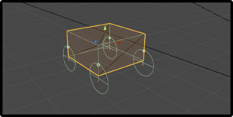
any vehicle in Unity is a combination of: 4 wheels colliders and 1 car collider.

WheelConllider

1) AxleInfo

AxleInfo represents the pair of wheels, so for 4-wheel vehicle, there are two AxleInfo objects.

1
2
3
4
5
6
7
8
9
10

struct AxleInfo 
{
  WheelCollider  left ;
  WheelCollider right; 
  GameObject leftVisual ;
  GameObject  rightVisual ;
  bool motor ;    #enable movement of this wheel pair
  bool steering ; # enable rotation of this wheel pair 
  float brakeBias = 0.5f; 
}

2) core parameters

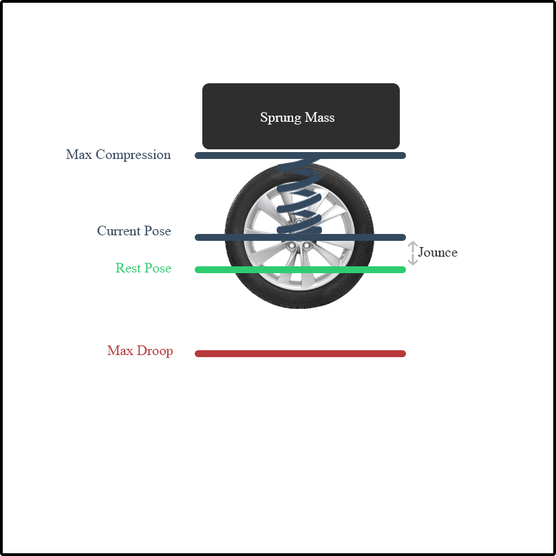
• wheel damping rate

• suspension distance

• Force apply point distance (where ground force act on wheel)

• suspension spring

• forwardSlip(slip angle), tire slip in the rolling(tractional) direction, which is used in calculating torque

• sidewaySlip, the lateral direction slip, which leads to stability issue.

3) visualization

the WheelCollider GameObject is always fixed relative to the vehicle body, usually need to setup another visual GameObject to represent turn and roll.

implementation from lg-sim

1
2
3
4
5
6
7
8
9
10
11

void ApplyLocalPositionToVisuals(WheelCollider collider, GameObject visual)
    {
        Transform visualWheel = visual.transform;
        Vector3 position;
        Quaternion rotation;
        collider.GetWorldPose(out position, out rotation);
        visualWheel.transform.position = position;
        visualWheel.transform.rotation = rotation;
    }

4) WheelCollider.ConfigureVehicleSubsteps

1

public void ConfigureVehicleSubsteps(float speedThreshold, int stepsBelowThreshold, int stepsAboveThreshold);

Every time a fixed update happens, the vehicle simulation splits this fixed delta time into smaller sub-steps and calculates suspension and tire forces per each smaller delta. Then, it would sum up all resulting forces and torques, integrate them, and apply to the vehicle’s body.

5) WheelCollider.GetGroundHit
return the ground collision data for the wheel, namely WheelHit

wheel friction curve

for wheels’ forward(rolling) direction and sideways direction, first need to determine how much the tire is slipping, which is based on speed difference between the tire’s rubber and the road,
then this slip is used to find out the tire force exerted on the contact point

the wheel friction curve taks a measure of tire slip as an Input and give a force as output.

The property of real tires is that for low slip they can exert high forces, since the rubber compensates for the slip by stretching. Later when the slip gets really high, the forces are reduced as the tire starts to slide or spin

1) AnimationCurve
unity official

store a collection of Keyframes that can be evaluated over time

vehicleController() in lg-sim

1) the controllable parameters:

1
2
3
4
5
6

currentGear 
currentRPM
currentSpeed 
currentTorque
currentInput 
steerInput

2) math interpolate function used

Mathf.Lerp(a, b, t)

a -> the start value

b -> the end value

t -> the interpolation value between start and end

3) fixedUpdate()

1
2
3
4
5
6
7
8
9
10
11
12
13
14

// cal trace force by rigidbody
rigidbody.AddForce(air_drag)
rigidbody.AddForce(air_lift)
rigidbody.AddForceAtPosition(tire_drag, act_position)
// update current driving torque
currentTorque = rpmCurve.Evalue(currentRPM / maxRPM) * gearRaion * AdjustedMaxTorque 
// apply torque 
// apply traction control
// update speed
currentSpeed = rigidbody.velocity.magnitude
// update fuel info
fuelLevel -= deltaConsumption
// update engine temp
// update turn signal light

4) ApplyTorque()

1
2
3
4
5
6

float torquePerWheel = accelInput * (currentTorque / numberofWheels) 
foreach(axle in axles):
	if(axle.left.motor):
		axle.left.motorTorque = torquePerWheel
	if(axle.right.motor):
		axle.right.motorTorque = torquePerWheel

5) TractionControl()

1
2
3
4
5
6
7
8
9
10
11
12

TractionControl()
{
	AdjustTractionControlTorque(axle.hitLeft.forwardSlip)
}
			
AdjustTractionControlTorque(forwardSlip)
{
   if(forwardSlip > SlipLimit)
	tractionMaxTorque -= 10 
   else 
        tractionMaxTorque += 10 
}

in lg-sim, the VD model is still simple, as there is only traction/logitudional control.

refer

add equation in markdown

wheelcollider doc

whell collider official

whellcollider tutorial

低速发展和高附加值

昨天看到一篇比较中欧(美)国家差异的帖子：北欧国家是如何保持高福利的。非常有意思的一个概念：高附加值，低发展速度的行业。

这些国家有一些传统强势行业。很有意思的是，印象中的传统行业，比如农业、畜牧业、纺织、手工业等等，跟高科技、现代化很远，似乎是非洲国家的土著人干的活儿。相比，在国内，互联网、技术创业、地产、金融、mba营销、国际贸易等才是时尚。

早年在农业大学，对以色列强大的现代农业是有所耳闻的。只是没有这种洞察力，现代化的传统行业与国民福利之间还有这样的隐形关系。

相比，美国的农业、畜牧业等传统行业很不错；美国也引领科技、金融这些时尚的行业。在美国生活的人民确是有了进退的余地。向左，可以退居大农村；向右，可以进军纽约、硅谷当金融、科技新贵。

国家的选择看似主动，也是现实的驱动。国家可以集中发力在互联网、金融、创业等方面做的很有声有色，但与此同时，传统的制造业，典型低发展速度，需要长期积累，国家发力也解不了。比如，汽车发动机、精密仪器、芯片制造等。

制造业在国内的标签是低附加值，资本不愿意进入，国家队发力也没气色。然而经过了这些长期积累的国家，比如欧洲小国瑞士、德国，制造业出口完全是高端制造的典范。而且马太效应显著，让这些欧洲国家不需要社会剧烈的经济变动，不需要老百姓担心行业变动、反倒一年还有20天带薪假。政府和人民都其乐融融，有时候看北欧人的生活，建筑、厨房、国家公园、办公环境、甚至监狱，简直像在童话里；报道一个小小的新闻，似乎都要惊动整个镇子上的人一样，这里简直就生活在像伊甸园。

而中国总是一片火热的场景，5年大力发展基建、5年大力吹捧全国创业、又5年搞工业互联网。国家没有消停，老百姓有人欢喜有人愁。

中国没有先发优势，在这些传统行业缺少长期积淀，强行进入既不不讨资本喜欢，也不讨人喜欢。比如报道，西安火箭研究员工资20万；大国重器的老焊工，无数荣誉奖章，一个月才一万多，在北京买不起房；国家队出动安利中小企业贷款，但银行就是宁愿带给亏损的国企，也不给需要钱的中小企业。

对于这些需要长期资本补血，短期回报低，才能形成壁垒的传统行业。在这个资本、市场竞争相对成熟的年代，确实比100年前，搞种植、搞养殖，或西门子、博世等制造业刚出道积累行业(非金钱资本)“资本”要困难的多。似乎印证了上周接触深圳汽车电子行业的感触，一个词：活着。根本谈不上行业积累。

可以说，北欧国家以及北美国家，因为上几代人的积累，给他们留下的行业遗产、社会制度遗产，才允许他们活的这么滋润。相比，中国没有上几代人的遗产，又进入了成熟资本市场的21世纪，所以，是压力也是机遇。去发掘新世纪的矿吧。

对这个大环境的从业者而言，选择农业、传统制造业，也确实不聪明。干着比人累的活儿，挣得比人少，社会还不待见。年轻人选择行业要识大局。相比，这个时代热的东西，确实该多关注。存在即合理。

工程师的心态

国内有些企业家喜欢讲情怀，吹“工匠精神”, 结果把自己作死了。而华为这样的企业，可以拿高薪，也是加班拿命换的。能够心安理得的当一名工程师，不需要为生计、价值实现、社会待见操心的，只会在这些“低速、高附加值”的欧美公司。一个国家的企业能进化到这种形态，基本是社会稳定，企业稳定，developed，达到了一个最佳平衡点，再投资也不会增加收益，每个岗位都相对稳定，组织内部管理效能达到最优，系统的规范化远超过个人能力，所以每个员工心安理得，做好自己份内的事就好。剩下的时间，享受生活，或者出于兴趣爱好，搞点车库创业都不在话下。

相比，国内的市场还在巨变当中，没有一家企业已经进化到developed，企业组织系统还不成熟，个人能力还能发挥显著价值，那老老实实当工程师的，在还在发生资源重组系统里，就会被挤到最底层。所以，不要怪国内的年轻人心态不正。因为这个时代，传统技工不会长在国内，国内应该培养属于这个时代的阶层和行业。想跟欧美，比工匠精神，确实是拿短处跟人家的长处比。