Serious Autonomous Vehicles


  • Home

  • Archives

  • Tags

  • Search

driving scenarios on-going

Posted on 2020-03-04 |

Euro NCAP driving scenarios

Adaptive Cruise Control(ACC)

ACC is tested in an extended version of AEB. these systems are designed to automatically adapt the speed when approaching a slower moving vehicle or noe that is braking. notification, not all systems perform well with stationary obstacles.

  • a slow moving vehicle test

  • a stationary obstacle(e.g. vehicle) test

autonomous emergency braking(AEB)

AEB pedestrain

  • an adult pedestrain running from the driver’s side of the vehicle

  • an adult walk from the passenger’s side

  • a child runs from between parked cars on the passenger’s side of the car

  • pedestrain walking in the same direction as the vehicle algnedwith the centre of vehicle

  • pedestrain walking in the same direction as the vehicle offset to one side

AEB cyclist

  • cyclist is crossing the vehicle’s path

  • cyclist is travelling in the same direction

Euro NCAP gives greatest reward if a collision is completely avoided; in some case, if AEB is unable to stop the vehicle completely, still give some points.

lane keeping assist(LKA)

  • lane centering, a good ADS should continue to support the driver during the manoeuvre and will not resist the driver or deactivate.

  • cut-in test, a npc from adjacent lane merges into the current lane

  • cut-off test, a npc leaves the current lane abruptly to avoid a stopped vehicle ahead

  • swerve around a small obstacle test

  • speed assistance test, to use map data and/or data from sensors to identify the local speed limit

NHTSA driving scenarios

a previous blog design scenarios in ADS simulation is based on NHTSA.

forward collision prevention

  • Forward collision warning
  • AEB
  • pedestrain AEB
  • Adaptive lighting

backing up & parking

  • rear automatic braking
  • backup camera
  • rear cross traffic alert

lane & side assist

  • lane departure warning
  • lane keeping assist
  • blind spot detection
  • lane centering assist

maintaing safe distance

  • traffic jam assist
  • highway pilot
  • ACC

Matlab Driving Scenario samples

AEB (for vulnerable road users)

  • AEB_Bicyclist_Longitudinal_25width, at collision time, the bicycle is 25% of the way across the width of the ego vehicle.

  • AEB_CCRb_2_initialGap_12m, a car-to-car rear braking(CCRb) scenario where the ego rear hit a braking agent. the deceleration is 2 m/s^2 with initial gap 12m

  • AEB_CCRm_50overlap, a car-to-car rear moving(CCRm) scenario, where the ego rear hits a moving vehicle. at collisio ntime, the ego overlaps with 50% of the width of the moving vehicle

  • AEB_CCRs_-75overlap, a car-to-car stationary(CCRs) sceanrio, where the ego rear hits a stationary vehicle. at collision time, the ego overlaps with 75% of the width of the stationary vehicle. when the ego is to the left of the other vehicle, the percent overlap is negative
  • AEB_Pedestrain_Farside_50width, the ego collides with a pedestrain who is traveling from the left side(far side, assuming vehicle drive on right side of the road). at collision time, the pedestrain is 50% of the way across the width of the ego

  • AEB_PedestrainChild_Nearside_50width, the ego collides with a pedestrain who is traveling from the right side(near side), at collision time, the pedestrain is 50% of the way across the width of the ego

Emergency Lane Keeping(ELK)

  • ELK_FasterOvertakingVeh_Intent_Vlat_0.5, ego intentionally changes lanes but collides with a faster overtaking vehicle, the ego travels at a lateral velocity of 0.5m/s

  • ELK_OncomingVeh_Vlat_0.3, ego unintentionally changes lanes and collides with an oncoming vehicle, with ego’s lateral velocity of 0.3m/s

  • ELK_OvertakingVeh_Unintent_Vlat_0.3, ego unintentionally changes lanes, overtake a vehicle in the other lane and collides. the ego travles at a lateral velocity at 0.3m/s

  • ELK_RoadEdge_NoBndry_Vlat_0.2, ego unintentionally changes lanes and ends up to hte road edge, with lateral velocity at 0.2m/s

LKA

  • LKA_DashedLine_Solid_Left_Vlat_0.5

  • LKA_DashedLine_Unmarked_Right_Vlat_0.5

  • LKA_RoadEdge_NoBndry_Vlat_0.5

  • LKA_RoadEdge_NoMarkings_Vlat_0.5

  • LKA_SolidLine_Dashed_Left_Vlat_0.5

  • LKA_SolidLine_Unmarked_Right_Vlat_0.5

open source libs

  • Microsoft: autonomous driving cookbook

  • TrafficNet: an open scenario lib

  • Toyota: vehicle simulation unity toolkit

  • mathworks: github

  • sensetime: driving stero dataset

  • google: open simulator interface

  • cmu: ml4ad

scenarios in L2 vs L3+

scenarios in l2 is more like point in the whole driving manuevor, at a certain scenario/point, how the ADAS system response. while L3+ is a continously scenario, along each point during driving is part of the scenario, and inside which all kinds of l2 case scenario can happen. it does make sense to integrate l2 scenario planning response to l3+, which makes l3+ system more strict.

refer

2018 Automated driving test

mathworks: Euro NCAP driving scenarios in driving scenario designer

Euro NCAP roadmap 2025

nhtsa vehicle safety legacy doc

NHTSA driver assitance tech

Study and adaptation of the autonomous driving simulator CARLA for ATLASCAR2

implementing RSS model on NHTSA pre-crash scenarios

boto3 streamingBody to BytesIO

Posted on 2020-03-03 |

boto3 streamingBody to BytesIO

boto3 class into

  • A Session is about a particular configuration. a custom session:
1
2
3
session = boto3.session.Session()
ads = session.client('ads')
ads_s3 = session.resource('s3')
  • Resources is an object-oriented interface to AWS. Every resource instance has a number of attributes and methods. These can conceptually be split up into identifiers, attributes, actions, references, sub-resources, and collections.
1
obj = ads_s3.Object(bucket_name="boto3", key="test.mdf")
  • Client includes common APIs:
1
2
3
4
5
6
7
8
9
10
11
12
13
14
15
16
17
18
copy_object()
delete_object()
create_bucket()
delete_bucket()
delete_objects()
download_file()
download_fileobj()
get_bucket_location()
get_bucket_policy()
get_object()
head_bucket()
head_object()
list_buckets()
list_objects()
put_bucket_policy()
put_object()
upload_file()
upload_fileobj()
  • Service Resource have bucket and object subresources, as well as related actions.

  • Bucket, is an abstract resource representing a S3 bucket.

1
b = ads_s3.Bucket('name')
  • Object, is an abstract resource representing a S3 object.
1
obj = ads_s3.Object('bucket_name', 'key')

read s3 object & pipeline to mdfreader

there are a few try-and-outs. first is to streaming s3 object as BufferedReader, which give a file-like object, and can read(), but BufferedReader looks more like a IO streaming than a file, which can’t seek.

botocore.response.StreamingBody as BufferedReader

the following discussion is really really helpful:
boto3 issue #426: how to use botocore.response.StreamingBody as stdin PIPE

at the code of the StreamingBody and it seems to me that is is really a wrapper of a class inheriting from io.IOBase) but only the read method from the raw stream is exposed, so not really a file-like object. it would make a lot of sense to expose the io.IOBase interface in the StreamingBody as we could wrapped S3 objects into a io.BufferedReader or a io.TextIOWrapper.read() get a binary string . the actual file-like object is found in the ._raw_stream attribute of the StreamingBody class

1
2
3
4
import io
buff_reader = io.BufferedReader(body._raw_stream)
print(buff_reader)
# <_io.BufferedReader>

wheras this buff_reader is not seekable, which makes mdfreader failure, due to its file operate needs seek() method.

steam a non-seekable file-like object

stdio stream to seekable file-like object

so I am thinking to transfer the BufferedReader to a seekable file-like object. first, need to understand why it is not seekable. BufferedRandom is seekable, whereas BufferedReader and BufferedWriter are not. Buffered streams design: BufferedRandom is only suitable when the file is open for reading and writing. The ‘rb’ and ‘wb’ modes should return BufferedReader and BufferedWriter, respectively.

is it possbile to first read() the content of BufferedReader to some memory, than transfer it to BufferedRandom? which gives me the try to BufferedReader.read(), which basicaly read all the binaries and store it in-memoryA, then good news: in-memory binary streams are also aviable as Bytesio objects:

f = io.BytesIO(b"some in-memory binary data")

what if assign BytesIO to this in-memoryA. which really gives me a seekable object:

fid_ = io.BufferedReader(mf4_['Body']._raw_stream) ;
read_in_memory = fid_.read()
bio_ = io.BytesIO(read_in_memory);

then BytesIO object pointer is much more file-like, to do read() and seek().

refer

boto3 doc

boto3 s3 api samples

mdf4wrapper

iftream to FILE

what is the concept behind file pointer or stream pointer

using io.BufferedReader on a stream obtained with open

working with binary data in python

read binary file and loop over each byte

smart_open project

PEP 3116 – New I/O

ceph & boto3 introduction

Posted on 2020-02-28 |

ceph intro

A Ceph Storage Cluster requires at least one Ceph Monitor, Ceph Manager, and Ceph OSD (Object Storage Daemon)

ceph storage cluster

The Ceph File System, Ceph Object Storage and Ceph Block Devices read data from and write data to the Ceph Storage Cluster.

cluster operations

data placement

  • pools, which are logical groups for storing objects

  • Placement Groups(PG), PGs are fragments of a logical object pool

  • CRUSH maps, provide the physical topology of the cluster to the CRUSH algorithm to determine where the data for an object and its replicas should be stored, and how to do so across failure domains for added data safety among other things.

  • Balancer, a feature that will automatically optimize the distribution of PGs across devices to achieve a balanced data distribution

Librados APIs workflow

apis can interact with: Ceph monitor as well as OSD.

  • get libs

configure a cluster handling

  • the client app must invoke librados and connected to a Ceph Monitor
  • librados retrieves the cluster map
  • when the client app wants to read or write data, it creates an I/O context and bind to a pool
  • with the I/O context, the client provides the object name to librados, for locating the data.
  • then the client application can read or write data

Thus, the first steps in using the cluster from your app are to 1) create a cluster handle that your app will use to connect to the storage cluster, and then 2) use that handle to connect. To connect to the cluster, the app must supply a monitor address, a username and an authentication key (cephx is enabled by defaul

an easy way, in Ceph configuration file:

1
2
3
[global]
mon host = 192.168.0.1
keyring = /etc/ceph/ceph.client.admin.keyring

image

1
2
3
4
5
6
7
8
9
10
11
12
13
14
15
16
17
import rados
try:
cluster = rados.Rados(conffile='')
except TypeError as e:
print 'Argument validation error: ', e
raise e
print "Created cluster handle."
try:
cluster.connect()
except Exception as e:
print "connection error: ", e
raise e
finally:
print "Connected to the cluster."

python api, has default admin as id, ceph as cluster name, and ceph.conf as confffile value

creating an I/O context

RADOS enables you to interact both synchronously and asynchronously. Once your app has an I/O Context, read/write operations only require you to know the object/xattr name.

1
2
3
4
5
6
7
8
9
10
11
12
13
14
15
16
17
18
19
20
21
22
23
24
25
26
27
28
29
30
31
32
33
34
35
36
37
print "\n\nI/O Context and Object Operations"
print "================================="
print "\nCreating a context for the 'data' pool"
if not cluster.pool_exists('data'):
raise RuntimeError('No data pool exists')
ioctx = cluster.open_ioctx('data')
print "\nWriting object 'hw' with contents 'Hello World!' to pool 'data'."
ioctx.write("hw", "Hello World!")
print "Writing XATTR 'lang' with value 'en_US' to object 'hw'"
ioctx.set_xattr("hw", "lang", "en_US")
print "\nWriting object 'bm' with contents 'Bonjour tout le monde!' to pool 'data'."
ioctx.write("bm", "Bonjour tout le monde!")
print "Writing XATTR 'lang' with value 'fr_FR' to object 'bm'"
ioctx.set_xattr("bm", "lang", "fr_FR")
print "\nContents of object 'hw'\n------------------------"
print ioctx.read("hw")
print "\n\nGetting XATTR 'lang' from object 'hw'"
print ioctx.get_xattr("hw", "lang")
print "\nContents of object 'bm'\n------------------------"
print ioctx.read("bm")
print "Getting XATTR 'lang' from object 'bm'"
print ioctx.get_xattr("bm", "lang")
print "\nRemoving object 'hw'"
ioctx.remove_object("hw")
print "Removing object 'bm'"
ioctx.remove_object("bm")

closing sessions

1
2
3
4
5
print "\nClosing the connection."
ioctx.close()
print "Shutting down the handle."
cluster.shutdown()

librados in Python

data level operations

  • configure a cluster handle

To connect to the Ceph Storage Cluster, your application needs to know where to find the Ceph Monitor. Provide this information to your application by specifying the path to your Ceph configuration file, which contains the location of the initial Ceph monitors.

1
2
import rados, sys
cluster = rados.Rados(conffile='ceph.conf')
  • connect to the cluster
1
2
3
4
5
6
7
8
9
cluster.connect()
print "\nCluster ID: " + cluster.get_fsid()
print "\n\nCluster Statistics"
print "=================="
cluster_stats = cluster.get_cluster_stats()
for key, value in cluster_stats.iteritems():
print key, value
  • manage pools
1
2
3
4
5
cluster.create_pool('test')
pools = cluster.list_pools()
for pool in pools:
print pool
cluster.delete_pool('test')
  • I/O context

to read from or write to Ceph Storage cluster, requires ioctx.

1
2
3
ioctx = cluster.open_ioctx($ioctx_name)
#
ioctx = cluster.open_ioctx2($pool_id)

ioctx_name is the name of the pool, pool_id is the ID of the pool

  • read, write, remove objects
1
2
3
ioctx.write_full("hw", "hello")
ioctx.read("hw")
ioctx.remove_object("hw")
  • with extended attris
1
2
3
4
5
6
7
8
9
10
11
12
13
14
15
ioctx.set_xattr("hw", "lang" "en_US")
ioctx.get_xattr("hw", "lang")
```
* list objs
```python
obj_itr = ioctx.list_objects()
while True:
try:
rados_obj = obj_itr.next()
print(rados_obj.read())

RADOS S3 api

Ceph supports RESTful API that is compatible with basic data access model of Amazon S3 api.

1
2
3
4
5
PUT /{bucket}/{object} HTTP/1.1
DELETE /{bucket}/{object} HTTP/1.1
GET /{bucket}/{object} HTTP/1.1
HEAD /{bucket}/{object} HTTP/1.1 //get object info
GET /{bucket}/{object}?acl HTTP/1.1

Amazon S3

Simple Storage Serivce(s3) is used as file/object storage system to store and share files across Internet. it can store any type of objects, with simple key-value. elastic computing cluster(ec2) is Amazon’s computing service. there are three class in S3: servivce, bucket, object.

there are two ways to access S3, through SDK(boto), or raw Restful API(GET, PUT). the following is SDK way.

create a bucket

Put(), Get(), return all objects in the bucket. Bucket is a storage location to hold files(objects).

1
2
3
4
5
6
7
8
9
10
11
12
13
14
15
16
17
18
def create_bucket(bucket_name, region=None):
try:
if region is None:
s3_client = boto3.client('s3')
s3.client.create_bucket(Bucket=bucket_name)
else:
s3_client = boto3.client('s3', region_name=region)
location = {'LocationConstraint': region}
s3_client.create_bucket(Bucket=bucket_name,
CreateBucketConfiguration=location)
except ClientError as e:
logging.error(e)
return False
return True
response = s3_client.list_buckets()
for bucket in response['Buckets']:
print bucket

upload files

basically to upload a file to an S3 bucket.

1
2
3
4
5
6
7
8
9
10
11
12
13
def upload_file(file_name, bucket, object_name=None):
if object_name is None:
object_name = file_name
# Upload the file
s3_client = boto3.client('s3')
try:
response = s3_client.upload_file(file_name, bucket, object_name)
except ClientError as e:
logging.error(e)
return False
return True

upload_file() handles large files by splitting them into smaller chunks and uploading each chunk in parallel. which is same logic as ceph to hide the lower-level detail of data splitting and transfering.

upload_fileobj() accepts a readable file-like object, which should be openedin bin mode, not text mode:

1
2
3
s3 = boto3.client('s3')
with open("FILE_NAME", "rb") as f:
s3.upload_fileobj(f, "BUCKET_NAME", "OBJECT_NAME")

all Client, Bucket and Object have these two methods.

download files

download_file() a pair of upload files method, which accepts the names of bucket and object to download, and the filename to save the downloaded file to.

1
2
s3 = boto3.client('s3')
s3.download_file('BUCKET_NAME', 'OBJECT_NAME', 'FILE_NAME')

same as upload file, there is a read-only open method: download_fileobj().

bucket policy

1
2
3
4
5
6
s3 = boto3.client('s3')
result = s3.get_bucket_policy(Bucket='BUCKET_NAME')
bucket_policy = json.dumps(bucket_policy)
s3.put_bucket_policy(Bucket=bucket_name, Policy=bucket_policy)
s3.delete_bucket_policy(Bucket='BUCKET_NAME')
control_list = s3.get_bucket_acl(Bucket='BUCKEET_NAME')

get objects

1
2
obj_list = s3.list_objects(Bucket='bucket_name')
obj_cont = s3.get_object(Bucket='bucket_name', Key='file_key')

error: botocore.errorfactory.NoSuchKey: An error occurred (NoSuchKey) when calling the GetObject operation: Unknown

read objects through url (restful api)

through url path to get a file/object: https://<bucket-name>.s3.amazonaws.com/<key>

refer

ceph official doc

botocore official doc

boto3 github

amazon S3 example

GUI: create an S3 bucket and store objects in AWS

boto API access S3 object

from HPC to cloud (2) - distributed storage intro

Posted on 2020-02-27 |

常见分布式存储

背景

  • 块存储 vs 文件存储

文件存储读写慢,利于共享;块存储读写快,不利于共享。所有磁盘阵列都是基于Block块的模式,而所有的NAS产品都是文件级存储。物理块与文件系统之间的映射关系:扇区→物理块→逻辑块→文件系统。所以,文件级备份,需要一层一层往下查找,最后才能完成整个文件复制。

  • 对象存储 vs 块存储

富含元数据的对象存储使大规模分析成为企业的有吸引力的命题。对象存储也使得提供和管理跨越地理位置的存储变得相对经济。同时,块存储的属性使其成为高性能业务应用程序、事务数据库和虚拟机的理想选择,这些应用程序需要低延迟、细粒度的数据访问和一致的性能。块存储(云盘)只能被一个主机挂载。

  • 文件存储 vs 对象存储

对象存储(ceph, Linux block device)和文件系统(hdfs, gfs, restful Web API)在接口上的本质区别是对象存储不支持fread(), fwrite()类似的随机位置读写操作,即一个文件PUT到对象存储里以后,如果要读取,只能GET整个文件,如果要修改一个对象,只能重新PUT一个新的到对象存储里,覆盖之前的对象或者形成一个新的版本。对象存储的接口是REST风格的,通常是基于HTTP协议的RESTful Web API,通过HTTP请求中的PUT和GET等操作进行文件的上传即写入和下载即读取,通过DELETE操作删除文件。文件存储读写api如,file.open(); 对象存储读写api如 s3.open()。文件存储,多次读写;对象存储,一次写,多次读。对象存储的容量是无上限的;文件存储的容量达到一定上限,性能会极差。

对象存储,需要对原数据做解析吗?

存储类型

  • 块存储
    Direct Attach Storage(DAS), 每台主机服务器有独立的存储设备,各存储设备之间无法互通,需要跨主机存取。 Storage Area Network(SAN), 高速网络连接的专业存储服务器,与主机群通过高速i/o连结。

  • 文件存储
    Network Attached Storage(NAS), 连接在网络上并提供存取服务。采用NFS或CIFS命令集访问数据,以文件为传输协议,通过TCP/IP实现网络化存储,可扩展性好、价格便宜、用户易管理

  • 对象存储
    核心是将数据通路(数据读或写)和控制通路(元数据)分离,并且基于对象存储设备(Object-based Storage Device,OSD)构建存储系统。对象存储设备具有一定的智能,它有自己的CPU、内存、网络和磁盘系统. 一般配置metadata server(MDS)。

存储用例

  • 对象存储
    非结构化(文档、图像、视频等)、备份存档、大数据分析(无实时性)

  • 块存储
    比较适合数据库业务、虚拟机

  • 文件存储
    企业共享、hpc大数据分析、流媒体处理,web服务。

容器云

容器云架构

1
2
3
4
5
控制台门户(管理员入口)
saas()
paas(容器,微服务、中间件、cicd)
资源调度管理平台
iaas(计算、存储、网络),虚拟化提供资源池,
  • 物理机直接架构k8s

容器云与私有云搭建的硬件资源分开。

  • 虚拟层上支持k8s

容器部署在虚拟机上的原因:既需要容器,也需要虚拟机的环境。一般互联网公司倾向分开容器的资源 和 虚拟机的资源。不管是容器云,还是虚拟机,都会有一个web管理平台。考虑弹性升缩,vm更灵活。而如果容器直接部署在x86裸机上,如果没有容器的管理层,docker容器挂了,就无法恢复。

应用部署容器云 vs 私有云

  • 仿真计算,倾向容器环境

  • CI/CD开发工具、中间件,倾向容器环境

  • web server,倾向容器环境

  • sql,倾向物理机或虚拟机

参考

KingStack

UCloud

EasyStack

from HPC to cloud computing

Posted on 2020-02-25 |

HPC

Ansys HPC, OpenFoam in amazon EC2, rescale, these are some samples of current CAE applications in HPC cloud.

most CAE simulations, in nut, are solving large sparse matrix, either optmization or differential, which depends on famous linear equations solvers/libs, e.g. Petsc, libMesh, Intel Math Kernel e.t.c, inside which are implemented with message passing interface(MPI), share memory, or similar techs.

why MPI is a have-to in these applications? because the problem interested itself is so huge, which is so much computing heavily than windows office, WeChat.

as engineers want the result more preciesly, the problem interested dimension will increase more. e.g. a normal static stress analysis of vehicle engine is about 6 million elements, each of which will take 6 ~ 12 vertexes, and each vertex has 6 DoF, which gives about a kinematic matrix with size about 200 million x 200 million, no single PC can store this much data, and not even to do the matrix computing then.

so all these problems have to be running on super computers, or high-performance computer(HPC), which have more memory or CPU cores. beyond large memory and CPU cores, also need fast-speed network, as each CPU can do calculation really fast, 2 ~ 4 GHz, so if the system can’t feed data that fast, the CPUs are hungry, which is the third feature of HPC: Gb high-speed internal network.

as the NUMA/multi-core CPU architecture is popular now, to achieve the best performance from these chips is also a hot topic.

cloud

if taken HPC as centerlized memory and CPU cores(the Cathedral), then cloud is about distributed memory and CPU cores(the Bazaar). cloud is more Internet, to connected weak-power nodes anywhere, but totally has great power. the applications in cloud must be easy to decomposed in small pieces, so each weak-power node can handle a little bit. when coming to cloud computing, I’d think about Hadoop, OpenStack, and docker.

hadoop is about to analysis massive data, which is heavily used in e-commercial, social network, games. docker is the way to package small application and each of the small image can run smoothly in one node, which currently is call micro-serivce, which is exactly as the name said, MICRO. OpenStack take care virtualization layer from physical memory, cpu resources, which used about in public cloud, or virtual office env.

A or B

cloud is more about DevOps, as each piece of work is not difference from the single PC, but how to deploy and manage a single piece of work in a large cloud is the key, so develop and operations together. compare to HPC, both develop and operation needs professions.

cloud computing has extended to edge computing, which is more close to normal daily life, and more bussiness-valued; while HPC guys are more like scientist, who do weather forcast, rocket science, molecular dynamics e.t.c.

finally, the tech itself, cloud or HPC, has nothing to do with the bussiness world.

refer

cloudscaling: grid, hpc, cloud… what’s the difference

linkedin: supver computer vs cloud

mdf4 reader

Posted on 2020-02-24 |

read mdf4 in general

image

the most important “branch” in the tree is the list of data groups (DG block).

record used to store the plain measurement data, the records can either be contianed in one single “data” (DT) block, or distributed over several DT blocks using a “data list” block .

Each DG block has points to the data block, as well as necessary information to understand and decode the data.

the sub-tree of DG is channel group(CG) blocks and channel(CN) blocks.

record layout

each record contains all signal values which have the same time stamp, in the same channel. for different channel groups(CG), each record must start with a “record id”

image

the record layout of ID 1, will be described by one channel group, the record layout of ID 2 by another channel group. Both channel groups must be children of the DT block’s parent data group.

channels

Each channel describes a recorded signal and how its values are encoded in the records for the channel’s parent CG block.

vector APIs

which is licensed by vector

  • GetFileManager()
  • OpenFile()
  • GetChannelByName()
  • GetChannelGroup()
  • CreaterDataPointer()
  • GetRecordCount()
  • SetReadMode()
  • SeekPos()
  • GetPos()
  • GetTimeSec()
  • ReadPhysValueDouble(pChannle, &value, &isvalid)
  • ReadRawValueDouble(pChannel, &rawValue)
  • ReadPhysValueDouble(pChannel, &phyValue)
  • MultiReadPhysValueDouble(pChannel, valueBuffer, size, &read)

turbolab

ReadFileMF4 class:

  • Open()
  • Seek(pos)
  • Read(Size, Buffer)
  • Close()

CMdf4Calc class :

  • Cmdf4Calc(pChan, pblock)
  • Cmdf4Calc(pChan, mf4file)

cmf4DataGroup class:

  • GetRecord()
  • GetRawValueFromRecord()
  • GetValueFromRecord()

mdf4FileImport class :

  • ImportFile()
  • ReleaseFile()

I am not reading this C++ code.

asammdf

MDF class

  • init(name=None, ): name can be either string or BytesIO
  • filter(channels, )
  • get_group(index, channels=None, )
  • iter_channels(,)
  • iter_get(channel_name=None,group_id=None, group_index=None, )
  • iter_groups()
  • to_dataframe(), generate pandas DataFrame
  • whereis(channel_name)

MDF4 class

includes data_group, channel_group, channels, data_block, data_location, record_size e.t.c

  • get(channel_name=None, group=None, )
  • get_can_signal()
  • get_channel_name(group, index)
  • get_channel_unit(channel_name=Nont, group=None, )
  • get_master(index, data=None, ), return the master channel samples for given group
  • info()

the following are sub data blocks of MDF4:

  • Channel class
  • ChannelGroup class
  • DataGroup class
  • DataList class
  • DataBlock class
  • HeaderBlock class
1
2
mdf = MDF4("basic.mf4")
db_info = mdf.info()

all group, channel data is packages as python dict. the most exciting part, as asam-mdf can support BytesIO, which gives the way to read mdf files stores in Amazon S3:

1
2
3
4
5
6
7
8
9
10
11
12
13
14
15
16
17
18
19
20
21
22
23
24
25
26
27
28
29
30
31
32
33
34
35
36
37
38
39
40
41
42
43
44
45
46
47
48
49
50
51
52
53
54
55
56
57
58
mf4_ = obj_api.get_object("bucket_name", "sample.mf4")
fid_ = io.BufferedReader(mf4_['Body']._raw_stream) ;
read_in_memory = fid_.read()
bio_ = io.BytesIO(read_in_memory);
if bio_.seekable():
mdf_ = MDF(bio_)
mdf_.info()
```
### installation of asam-mdf
* [install pandas](https://www.pypandas.cn/en/docs/installation.html#installing-using-your-linux-distribution’s-package-manager)
`python3 -m pip install pandas` (not working)
`sudo apt-get install python3-pandas`
* [install canmatrix](https://canmatrix.readthedocs.io/en/latest/installation.html)
`sudo python3 setup.py install`
* install pathlib2
`sudo -H pip3 install pathlib2 `
if `WARNING: pip is being invoked by an old script wrapper. This will fail in a future version of pip.`
using: `sudo -H python3 -m pip install(包名)`
## [mdfreader](https://github.com/ratal/mdfreader)
which is open source LSP licensed. and the APIs are clear about getChannels, and read data from each channel, which was my first choice. but later found out it's difficult to support streamIO input, which was the best format I can reached from Amazon S3 pipeline.
##### MdfInfo
* read_info()
* list_channels()
##### Mdf
* read()
* filter_channel_names()
* get_channel_data()
* get_channel_unit()
* keep_channels()
```python
import mdfreader
filename="basic.mf4"
file_info=mdfreader.MdfInfo()
channels = file_info.list_channels(filename)
print(channels)
file_pointer = mdfreader.Mdf(filename)
keys_ = file_pointer.keys()
for k_ in keys_:
chan1 = file_pointer.get_channel_data(k_)
print(chan1)

python necessary

buffered io

binary I/O, usually used in following:

1
2
3
f = open("mdf_file", "rb")
type(f)
<type '_io.BufferedReader'>

open(file, mode=’r’, buffering=-1, encoding=…)

ifmode='b', the returned content is bytes object, can’t encoding. if buffereing is not setted, for binary file with buffering with a fixed length. when with mode='w/r/t, it returns io.TextIOwrapper, if mode=rb, it returns io.BufferedReader, else if mode=wb, it returns io.BufferedWriter, else mode=wrb, it returns io.BufferedRandom. check here

dict built-in funs

1
2
3
4
5
6
7
8
9
10
cmp(dict1, dict2) ;
len(dict)
str(dict)
dict.clear()
dict.get(key)
dict.has_key(key)
dict.items()
dict.keys()
dict.values()
pop(key)

a bit about readers

a few years ago I was in CAE field, dealing with different kind of CAE format, e.g .nas. during that time, there is a similar need to have a file transfer from vendor specified format to python format e.t.c.

so now it comes again, which is funny to know adapters in CAE and autonomous driving design.

refer

asammdf API doc

asam mdf4 doc

gpu rendering in k8s cloud

Posted on 2020-02-21 |

background

to deploy simulation in docker swarm, there is a hurting that GPU rendering in docker requires a physical monitor(as $DISPLAY env variable). which is due to GeForece(Quadro 2000) GPUs, for Tesla GPUs there is no depends on monitor. really intertesting to know.

there were two thoughts how to deploy simulation rendering in cloud, either a gpu rendering cluster, or a headless mode in container cluster.

unity rendering

unity rendering pipeline is as following :

  • CPU calculate what need to draw and how to draw

  • CPU send commands to GPU

  • GPU plot

direct rendering

for remote direct rendering for GLX/openGL, Direct rendering will be done on the X client (the remote machine), then rendering results will be transferred to X server for display. Indirect rendering will transmit GL commands to the X server, where those commands will be rendered using server’s hardware.

1
2
direct rendering: Yes
OpenGL vendor string: NVIDIA

Direct Rendering Infrasturcture(DRI) means the 3D graphics operations are hardware acclerated, Indirect rendering is used to sya the graphics operations are all done in software.

DRI enable to communicate directly with gpus, instead of sending graphics data through X server, resulting in 10x faster than going through X server

for performance, mostly the games/video use direct rendering.

headless mode

to disable rendering, either with dummy display. there is a blog how to run opengl in xdummy in AWS cloud; eitherwith Unity headless mode, When running in batch mode, do not initialize graphics device at all. This makes it possible to run your automated workflows on machines that don’t even have a GPU. to make a game server running on linux, and use the argument “-batchmode” to make it run in headless mode. Linux -nographics support -batchmode is normally the headless flag that works without gpu and audio hw acceleration

GPU container

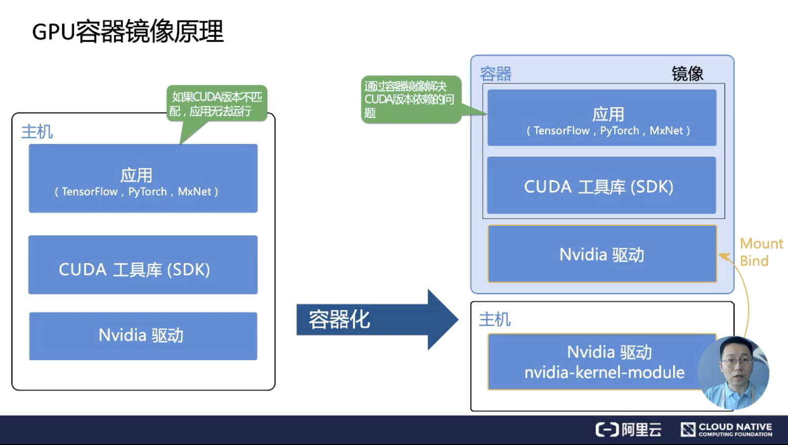
a gpu containeris needs to map NVIDIA driver from host to the container, which is now done by nvidia-docker; the other issue is gpu-based app usually has its own (runtime) libs, which needs to install in the containers. e.g. CUDA, deep learning libs, OpengGL/vulkan libs.

image

k8s device plugin

k8s has default device plugin model to support gpu, fpga e.t.c devices, but it’s in progress, nvidia has a branch to support gpu as device plugin in k8s.

nvidia docker mechanism

when application call cuda/vulkan API/libs, it further goes to cuda/vulkan runtime, which further ask operations on GPU devices.

cloud DevOps

simulation in cloud

so far, there are plenty of cloud simulation online, e.g. ali, tencent, huawei/octopus, Cognata. so how these products work? all of them has containerized. as our test said, only Tesla GPU is a good one for containers, especially for rendering needs; GeForce GPU requires DISPLAY or physical monitor to be used for rendering.

cloud vendors for carmakers

as cloud simulation is heavily infrastructure based, OEMs and cloud suppliers are coming together:

  • FAW -> Ali cloud
  • GAC -> Tencent Cloud
  • SAC -> Ali cloud / fin-shine
  • Geely -> Ali cloud
  • Changan -> Ali cloud
  • GWM -> Ali cloud
  • Xpeng, Nio (?)
  • PonyAI/WeRide (?)

obviously, Ali cloud has a major benefit among carmakers, which actually give Ali cloud new industry to deep in. traditionally, carmakers doesn’t have strong DevOps team, but now there is a change.

we can see the changing, as connected vehicles service, sharing cars, MaaS, autonomous vehicles are more and more requring a strong DevOps team. but not the leaders in carmakers realize yet.

fin-shine

SAC cloud, which is a great example for other carmakers to study. basically they are building the common cloud service independently.

  • container service <– k8s/docker
  • storage <– hdfs/ceph
  • big data <– hadoop/sql
  • middleware
  • applications <– AI, simulation

it’s an IP for SAC, but on the other hand, to maintain a stable and user-friendly cloud infrastructure is not easy at all.

refer

docker blender render cluster

nvidia vgpu

using GPUs with K8s

K8S on nvidia gpus

openGL direct hardware rendering on Linux

runinng carla without display

tips for runing headless unity from a script

Unity Server instance without 3d graphics

a blog: nvidia device plugin for k8s

k8s GPU manage & device plugin mechanism

review-apollo (2).md

Posted on 2020-02-17 |

review apollo (2)

EMPlanner

in review apollo(1), we had went through perception, prediction and part of planning module. the ADS planning problem can be summaried with a few input conditions, we can get a few drivable driving path, now EMPlanner, here need to find out the best one.

input conditions:

  • perception and prediction obstacles and its future(in 5s) trajectory

  • current road status, e.g. special area, pedestrain cross e.t.c.

both path and speed need to be planned or optimized. the core of EMPlanner is Dynamic programming(DP), which is an classic algorithm to search the global optimized solution. the DP garantee each sub-group best solution accumulated to the final global best solution.

PathOptimizer

the DP used in path optimizer basic processes:

starting from current location, in every time, move in x-direction about next n meters(to next location), and sample in y-direction at the next location, calcuate the cost from current location to each of the sampling point at the next location, and save cost value for each path for this sub path segment. (this is the different from DP to greedy algorithm), finally we retrieve all the cost values tables for each sub-path, and get the final best solution for the whole path.

a few question about DP here:

  • how long in x-direction need to plan ?

    KMinSampleDistance = 40.0
    
  • what size of the interval in x-direction is good ?

1
step_length = math::Clamp(init_point.v() * SamplePointLookForwardTime, config_.step_length_min(), config_.step_length_max());
  • how many sample points in y-direction is needed ?
1
num_sample_per_level = config_.sample_points_num_each_level();
  • how to sample in y-direction and x-direction ?

which is case by case, depends on the ego’s maneuver as well as the lanes info.

basically, we had RouteSegments/ReferenceLine set, which includes the filtered referencelines for ego vehicle. for each referenceLine, we can calcuate the cost, then figure out the min cost referenceline as planning module’s output.

1
2
3
4
5
6
7
8
9
10
11
12
13
14
15
16
17
18
19
20
21
22
23
24
25
26
EMPlanner::Plan(&start_point, *frame)
{
foreach reference_line_info in frame->reference_line_info():
PlanOnReferenceLine();
}
EMPlanner::PlanOnReferenceLine(start_point, frame, reference_line_info){
foreach optmizer in tasks_ :
ret = optmizer->Execute(frame, reference_line_info);
}
PathOptimizer::Execute(*frame, *reference_line_info){
ret = Process(speedData, reference_line, start_point, path_data);
}
DpPolyPathOptimizer::Process(SpeedData, ReferenceLine, init_point, path_data){
dp_road_graph.FindPathTunnel();
}
DPRoadGraph::FindPathTunnel(init_point, &obstacles, *path_data){
CalculateFrenetPoint(init_point, &init_frenet_frame_point_);
GenerateMinCostPath(obstacles, &min_cost_path);
foreach point in min_cost_path:
frenet_path.append(transfer(point));
path_data->SetFrenetPath(frenet_path);
}

point2point cost calcualation

e.g. from the left interval sample points(in y-direction) to current interval sample points(in y-direction).

during this cost calcuation, consider pathCost, staticObstacleCost and DynamicObstacleCost.

1
2
3
4
5
TrajectoryCost::Calculate(){
total_cost += CalculatePathCost();
total_cost += CalculateStaticObstacleCost();
total_cost += CalculateDynamicObstacleCost();
}
  • UpdateNode()
1
2
3
4
5
6
7
8
9
10
DPRoadGraph::GenerateMinCostPath(){
for(level=1; level < path_waypoints.size(); ++level){
level_points = path_waypoints[level]; //all sample points in y-direction at current level
for(i=0; i<level_points.size(); ++i){
cur_point = level_points[i];
UpdateNode(prev_dp_points, level, &trajectory_cost, &cur_point);
}
}
}
  • PathCost

from each point at prevous level to current point at current level, consider the length, 1st order(speed), 2sec order(acc) should be smooth, can give a 5th-order polyfit, same as what’d done in referenceLine smoother. for each interval/curve polyfit(by curve.Evaluate()), we can re-sampling it more density, so at each new sampling point, calculate its (position, speed, acc)l, dl, ddl

1
2
3
4
5
6
7
8
9
10
11
12
13
14
15
16
17
18
19
20
21
22
23
24
25
26
27
28
29
30
TrajectoryCost::CalculatePathCost(curve, start_s, end_s, curr_level){
foreach sampling_point in (end_s - start_s):
l = curve.Evalaute(0, sampling_point)
// cost from l
path_cost += l * l * config_.path_l_cost()
// cost from dl
dl = curve.Evaluate(1, sampling_point)
path_cost += dl * dl * config_.path_dl_cost()
// cost from ddl
ddl = curve.Evaluate(2, sampling_point)
path_cost += ddl * ddl * config_.path_ddl_cost()
}
```
* StaticObstacleCost
StaticObstacleCost() used the same idea from PathCost, basically, to resampling the interval, and calculate a cost on each of the sampling point.
```c++
TrajectoryCost::CalculateStaticObstalceCost(curve, start_s, end_s){
foreach curr_s in (end_s - start_s):
curr_l = curve.Evaluate(0, curr_s, start_s);
foreach obs_boundary :: static_obstacle_boundaries:
obstacle_cost += GetCostFromObs(curr_s, curr_l, obs_boundary);
}
TrajectoryCost::GetCostFrmObs(){
delta_l = fabs(adc_l - obs_center);
obstacle_cost.safety_cost += config_.obstacle_collision_cost() * Sigmoid(config_.obstacle_collision_distance() - delta_l) ;
  • DynamicObstacleCost
1
2
3
4
5
6
7
8
9
10
11
TrajectoryCost::CalculateDynamicObstacleCost(curve, start_s, end_s){
foreach timestamp:
foreach obstacle_trajectory in dynamic_obstacle_boxes_:
obstacle_cost += GetCostBetweenObsBoxes(ego_box, obstacle_trajectory.at(timestamp));
}
TrajectoryCost::GetCostBetweenObsBoxes(ego_box, &obs_box){
distance = obstacle_box.DistanceTo(ego_box);
if(distance > config_.obstacle_ignore_distance())
return obstacle_cost ;
obstacle_cost.safety_cost += ( config_.obstacle_collision_cost() + 20) * Sigmoid(config_.obstacle_collision_distance() - distance);

static obstacles cost calculating is like one space-dimension, only consider cost from the fixed/static obstacle to the fixed sampling points. for dynamic obstacles case, as the obstacle is moving, so we need a time-dimension, to calculate the cost at each time interval, from the current obstacle location to the fixed sampling points.

for dynamic obstacle cost, there is a risk cost (20), which need to take care.

min cost path

we got the cost matrix from the start_s level to the target_s/final level. but the final level in y-direction has 7 sampling points, all of which are drivable. so backward propagation, to get the best path (or a NODE in DAG)

1
2
3
4
DPRoadGraph::GenerateMinCostPath(){
for(cur_dp_node : graph_nodes.back()){
fake_head.UpdateCost()
}

SpeedOptimizer

the previous PathOptimier give the best (s, l) location of ego should arrived at each interval section along the referenceline. so what’s the best speed to reach these interval section ?

to do speed optimzier, two parts:

  • constraint speed conditions, e.g. speed limit, upper/lower boundary of drivable area along the refereneline due to obstacle trajectory

  • speed planning

BoundaryMapper()

for each obstalce’s trajectory, sampling in time-dimension, if its trajectory has overlapped with ego’s trajectory, mark the boundary box.

1
2
3
4
5
6
7
8
9
10
11
12
13
14
15
16
17
18
StBoundaryMapper::CreateStBoundary(){
foreach trajectory_point in trajectory:
obs_box = obstacle.GetBoundingBox(trajectory_point);
for(path_s=0.0, path<s < discretized_path.Length(); path_s += step_length){
curr_adc_path_point = discretized_path.EvaluateUsingLinearApproximation();
if( CheckOverlap(curr_adc_path_point, obs_box, st_boundary_config_.boundary_buffer()) )
{
}
}
}
// only when obs trajectory overlapped with ego's trajectory
StBoundaryMapper::MapWithDecision(path_obstacle, decision){
boundary = StBoundary::GenerateStBoundary(lower_points, upper_points);
path_obstacle->SetStBoundary(boundary);
// assign different boundary type
}

SpeedLimitDecider

  • speed limit

  • centripetal acc limit

  • centripetal force limit

DpStGraph::Search

so far we have info from boundaryMapper, which tells lower_s and upper_s of safe driving area along reference line, excluding the overlaping area of obstacle’s trajectories; as well as speed limit. so now in the driving safe area, which speed ego should take at each point is also done by DP, speed can be represent in time-space two dimension, in a T-S table.

so speed DP can transfer to find the min cost [T,S] althrough the whole planning drive path.

1
2
3
4
5
6
7
8
9
10
11
12
13
14
15
16
17
18
19
20
21
22
23
24
25
26
27
28
29
30
31
32
33
DpStGraph::Search(speed_data){
InitCostTable().ok();
CalculateTotalCost().ok();
RetriveSpeedProfile(speed_data).ok();
}
```
### QpSplineSpeedOptimizer
DPSpeedOptimizer output the value pair of (time, location)(t, s) at each interval, then can get the velocity, acc, angular velocity by differencial among the neighbor intervals. QPSpline is a better way to get a polyfit 2nd-order smoothed speed profile along the referenceLine, which is higher-precision than DP.
### SpeedOptimizer and PathOptimizer fusion
PathOptimizer outputs driving path in (accumulated_distance, section_direction distance)(s, l), SpeedOptimizer outputs driving path in (time, accumulated_distance)(t, s). now to get the best/optmized path along the referenceLine, need combine these two outputs.
```c++
for(cur_rel_time=0.0; cur_rel_time < speed_data_.TotalTime(); cur_rel_time += TimeSec){
speed_data_.EvaluateByTime(cur_rel_time, &speed_point);
if(speed_point.s() > path_data_.discretized_path().Length()) break;
path_data.GetPathPointWithPathS(speed_point.s(), &path_point);
path_point.set_s(path_point.s() + start_s);
trajectory_point.mutable_path_point()->CopyFrom(path_point);
trajectory_point.set_v(speed_point.v());
trajectory_point.set_a(speed_point.a());
trajectory_point.set_relative_time(speed_point.t() + relative_time);
ptr_discretized_trajectory->AppendTrajectoryPoint(trajectory_point);
}

the above fusion is on one ReferenceLine, for all referenceLine, we can reach out the min cost referenceline as following:

Frame::FindDriveReferenceLineInfo(){
    foreach reference_line_info in reference_line_info_ :
        if(reference_line_info.IsDrivable() && reference_lien_info.Cost < min_cost){
            drive_reference_line_info_ = &reference_line_info;
            min_cost = reference_line_info.Cost();
    }

    return drive_reference_line_info_ ;
}

Planning in summary

Planning module has three components, ReferenceLineProvider, Frame and EMPlanner. Frame has ReferencelineInfo, which has everything about once-time planning, including the min-cost ReferenceLineInfo from EMPlanner. EMPlanner do DP and QP for PathPlan and SpeedPlan, seperately, which give a best driving path for each RefereneLine. in the whole, we can reach out the global best(min-cost) referenceLine from EMPlanner, and store back in Frame.

Control

Control module readin the planning ReferenceLine (Trajectory, VehicleStatus) and Localization, output control command.

ControlComponent::Proc(){
    chassis_msg = chassis_reader_->GetLatestObserved();
    OnChassis(chassis_msg);
    trajectory_msg = trajectory_reader_-> GetLatestObserved();
    localization_msg = localization_reader_-> GetLatestObserved();

    status = ProduceControlCommand(&control_command);
    control_cmd_writter_->Write();
}

simulation

simulation is a system level verification/test tool, there are a few topics:

simulate the world

how to make a virtual world in simulation, quickly, easily, close to real and massively deploy-friendly.

currently most commericial tools, e.g. PreScan, CarMaker, are supporting well real map(.osm), and on-line/distributed/cloud service, which is good way.

a few pioneers are trying to make the virtual world by 3D build through image/point cloud scanning. which is maybe the closest way to the physical world, but need large computing resource.

integrate ADS system

how to integrate ADS system to simulation, easily.

most simulation software/platform is independent from ADS core.

for in-house prototype team, they both develop ADS and simulate in Matlab. which is pretty common in most OEM teams.

in product phase, it’s common to package ADS core as ros node, and talk to the simulation software by ROS.

friendly API

system level simulation has plenty of scenarios, requiring the simulation platform has friendly way to produce massively scenarios. including env, ego/npc behaviors, special cases e.t.c

most common APIs are Python and Matlab.

massively deployment

it’s back to the test purpose, simulation needs to cover as much as possible scenarios, which requires IT infrastructure to support massively deployment. e.g. cloud deployment

`

review apollo (1)

Posted on 2020-02-15 |

dig into Apollo/Daohu527 and YannZ/Apollo-Notes are some good summary of Apollo.

localization

rtk

!image

1
2
3
4
5
6
7
8
9
10
11
12
13
14
15
16
17
18
19
RTKLocalizationComponent::InitIO()
{
corrected_imu_listener_ = node_ ->CreateReader<localization::CorrectImu>();
gps_status_listener_ = node_ -> CreateReader<driver::gnss::InsStat>();
}
RTKLocalizationComponent::Proc(& gps_msg)
{
localization_->GpsCallback(gps_msg);
if(localization_->IsServiceStarted())
{
LocalizationEstimate localization;
localization_->GetLocalization(&localization);
localization_->GetLocalizationStatus(&localization_status);
PublishPoseBroadcastTopic(localization);
}
}

ndt

normal distribution transform(NDT) is to match our sensors view points compare to what we see on an existing map.

due to the view points from sensor may be a little off from the map, or the world might change a little between when built the map and when we record the view points.

so NDT will try to match view points to a grid of probability functions created from the map, instead of the map itself.

msf

perception

module overview

1
2
3
4
5
6
7
8
9
10
11
12
13
14
15
16
17
18
19
20
21
22
23
24
25
26
27
28
29
30
31
32
33
34
35
36
37
38
39
40
41
42
43
44
void Perception::RegistAllOnboardClass() {
RegisterFactoryLidarProcessSubnode();
RegisterFactoryRadarProcessSubnode();
RegisterFactoryFusionSubnode();
traffic_light::RegisterFactoryTLPreprocessorSubnode();
traffic_light::RegisterFactoryTLProcSubnode();
}
```
the data flow in perception has two ways, either ROS message send/subscribe, or shared data. Apollo design a `global map` data structure:
```c++
GlobalFactoryMap<string, map<string, ObjectFactory*> >
```
the first string element can be `SubNode` or `ShareData`.
e.g.
* lidar share data can stored as: `GlobalFactorMap[sharedata][LidarObjectData]`
* radar subnode data can stored as: `GlobalFactorMap[Subnode][RadarObjectData]`
#### DAG process
after ros subnode and shared data registered(not instance), [perception module create a DAG](https://github.com/YannZyl/Apollo-Note/blob/master/docs/perception/perception_software_arch.md)(directional acyclic graph) process, which includes subNode, Edge, and ShareData.
`Edge` defines start node and end node of the data flow. e.g. LidarProcessSubnode -> FusionSubnode.
* subnode init
```c++
DAGStreaming::InitSubnodes()
{
for(auto pair: subnode_config_map)
{
Sunode* inst = SubnodeRegisterer::GetInstanceByName(subnode_config.name());
inst->Init() ;
}
}
  • edge init
1
2
3
4
DAGStreaming::Init()
{
event_manager_.Init(dag_config_path.edge_config());
}

it’s easy to understand EventManager is used to register edge, as the data flow either by ros node or by share data is event driven. inside EventManager there are two variables:

event_queue_map <eventID, message_queue>

event_meta_map  <eventID, message_info>
  • shareData init
1
2
3
4
DAGStreaming::Init()
{
InitSharedData(dag_config.data_config());
}

each subnode and shareData is a separate ROS/data thread, which started after DAG process initialization finished, the run() process is the event loop:

1
2
3
4
5
6
7
8
9
10
11
12
13
14
15
16
17
18
19
20
DAGStreaming::Schedule()
{
for(auto& pair: subnode_map_)
{
pair.second->Start();
}
for(auto& pair : subnode_map_)
{
pair.second->Join();
}
}
Subnode::Run()
{
while(!stop)
{
status = ProcEvents();
}
}

Lidar process

  • hdmap ROI filter. basically compare the lidar cloud points to hdmap area, and filter out the cloud points outside of ROI.
  • CNN image segmentation, basically classfiy the point clouds as obstacles based on CNN.

  • obstacle minBox

  • obstalce tracking

  • lidar fusion

Lidar & Radar fusion

the data fusion ros node proces in the following way:

step1: collect sensor’s data

1
2
3
4
5
6
7
8
9
10
11
12
13
14
15
16
17
18
19
20
21
22
23
24
25
26
27
28
29
30
31
32
33
34
35
36
37
38
39
40
41
42
43
44
FusionSubnode::Process()
{
BuildSensorObjs(events, &sensor_objs);
fusion_->Fusion(sensor_objs, &objects+);
}
FusionSubnode::BuildSensorObjs(&events, std::vector<SensorObjects> * multi_sensor_objs){
foreach event in events:
{
if( event.event_id == lidar )
{
sensor_objects.sensor_type = VELODYNE ;
} else if ( event.event_id == radar){}
else if (event.event_id == camera) {}
else{return false;}
}
multi_sensor_objs->push_back(*sensor_objects);
}
```
step2: process sensors data
```c++
ProbabiliticFusion::Fuse(multi_sensor_objs, *fused_objs)
{
sensor_mutex.lock();
foreach sensor_objs in multi_sensor_objs:
{
sensor_manager_->AddSensorMeasurements(sensor_objs);
}
sensor_manager_->GetLatestFrames(fusion_time, &frames);
}
sensor_mutex.unlock();
sensor_mutex.lock();
foreach frame in frames:
FuseFrame(frame)
CollectFusedObjects(fusion_time, fused_objects);
sensor_mutex.unlock();

the data structure for sensor_type, timestamp and perceptioned obj is:

std::map<string sensorType, map<int64, SensorObjects> > sensors_;

sensors_[sensor_id][timestamp] return the sensor’s object at a special timestamp

for Lidar and Radar fusion, we get a frame list, each frame has the object list from both Lidar and Radar. basically, so far it is just matching Lidar objects to Radar objects, assiged to timestamp. Lidar objects and Radar objects are indepenent.

prediction

in Apollo, prediction module anticipatd the future motion trajectories of the perceived obstacles.

prediction subscribe to localization, planning and perception obstacle messages. when a localization update is received, the prediction module update its internal status, the actual prediction is triggered when perception sends out its perception obstacle messages, as following code :

1
2
3
MessageProcess:OnLocalization(*ptr_localization_msg);
MessageProcess:OnPlanning(*ptr_trajectory_msg)
MessageProcess:OnPerception(*ptr_perception_msg, &prediction_obstacles)

take a detail review of OnPerception as following:

1
2
3
4
5
6
7
8
9
10
MessageProcess:OnPerception(perception_obstacles, prediction_obstacles){
ptr_obstalces_container = ContainerManager::Instance()->GetContainer<ObstaclesContainer>();
ptr_trajectory_container = ContainerManager::Instance()->GetContainer<ADCTrajectoryContainer>();
EvaluatorManager::Instance()->Run(ptr_obstacles_container);
PredictorManager::Instance()->Run(perception_obstacles, ptr_trajectory_container, ptr_obstacles_container)

ContainerManager

used to instancialize an instance of the special container, which is used to store the special type of message. there are three types of contianer:

  • ObstaclesContainer

used to store obstalce info and its lane info. obstacle info coming from perception; its lane info coming from hd map and LaneGraph, LaneSequence and LaneSegment. check the explanation of ObstacleContainer

LaneGraph is namely the lane network. e.g. the pre/post lane, neighbor lane, or where the lane disappear. LaneSegment is the element/piece of discretization of the lane network, which has a start point and end point. LaneSequence is a set of all possible next lane choices from current lane, which is only based on the lane network and current obstacle velocity, rather than from planning.

  • PoseContainer

used to store vehicle world coord and the coord transfer matrix, velocity info e.t.c

  • ADCTrajectoryContainer

EvaluatorManager

what evaluator does, is to compute the probability of each laneSequence, the obstacle is either vehicle, or pedestrain or bicycle. to compute probability is with multi-layer predictor(MLP) model:

1
2
3
4
5
6
MLPEvaluator::Evaluate(obstacle_ptr){
foreach lane_sequence_ptr in lane_graph->lane_sequence_set:
ExtractFeatureValues(obstacle_ptr, lane_sequence_ptr, &feaure_values)
probability = ComputeProbability(feature_values);
}
  • ObstacleFeature

there are 22 dimensions, which are greate resources to understand a good prediction model in ADS.

these features includes, dimension, velocity, acc, direction of the obstacle, and relative position, angle to boundary lane e.t.c.

  • LaneFeature

since the laneSequence is already discritized as LaneSegment, for each lane Segment, Apollo calculate 4 features: the angle from lanePoint position to its direction vector; obstacle’s projected distance to laneSequence; the direction of lanePoint; the direction angle from lanePoint’s direction to obstacle’s direction.

for each LaneSequnce only calculate its first 40 features, namely the first 10 LaneSegment.

from 22 Obstacle features and 40 lane features, compute the probability of each LaneSequence.

PredictorManager

this is where we answer the predict question, where in the next 5 sec the obstacle located. after EvaluatorManager(), we get the probability of each LaneSequence. then choose the few LaneSequences with high probability, and predict a possible obstacle motion for each high-probability LaneSequence as well as with ADCTrajectory info from planning module.

1
2
3
4
5
6
7
8
9
10
11
12
13
14
15
16
17
18
19
20
21
22
23
24
25
26
27
PredictorManager::Run(perception_obstalces)
{
foreach obstacle in perception_obstacles:
predictor->Predict(obstacle)
foreach trajectory in predictor->trajectories():
prediction_obstacle.add_trajectory(trajectory)
prediction_obstacles.add_prediction_obstalce(prediction_obstalce)
}
```
basically for each obstacle, we do [prediction its next few seconds position](https://github.com/YannZyl/Apollo-Note/blob/master/docs/prediction/predictor_manager.md). there are a few predictors: MoveSequencePredictor, LaneSequencePredictor, FreeMovePredictor.
```c++
MoveSequencePredictor::Predict(obstacle)
{
feature = obstalce->latest_feature();
num_lane_sequence = feature.lane_graph().lane_sequence_size()
FilterLaneSequence(feature, lane_id, &enable_lane_sequence)
foreach sequence in feature.lane_sequence_set
{
DrawMoveSequenceTrajectoryPoints(*obstacle, sequence, &points)
trajectory = GenerateTrajectory(points)
trajectory.set_probability(sequence.probability());
trajectories_.push_back(trajectory)
}
}

why need prediction module

whether including motion prediction or not is based on the computing ability of ADS system. for low power system, the planning module update really high frequency, then there is no prediction, or prediction only need be considered in less than a few mic-sec; but for complex ADS system with low frequency update of planning, the ability to forsee the next few secs is very helpful.

Planning

!image

VehicleStateProvider

1
2
3
4
5
6
7
8
class VehicleStateProvider {
common::VehicleState vehicle_state_ ;
localization::LocalizationEstimate original_localization_ ;
Update();
EstimateFuturePosition();
}

P&C Map

update routing response

during PnC map, we need to query waypoints(in s, l coord), e.g. current vehicle position, target position, in which routing laneSegment.

  • get laneSegment info from routing response
1
2
3
4
5
6
7
8
PncMap::UpdateRoutingResponse(routing){
foreach road_segment in routing.road() :
foreach passage in road_segment.passage():
foreach lane in passage.segment():
{
all_lane_id.insert(lane.id());
}
}
  • query waypoints
1
2
3
RouteSegments::WithinLaneSegment(&lane_segment, &waypoint){
return lane_segment.lane->id().id() == waypoint.id() && waypoint.s() >= lane_segment.start_s && waypoint.s() <= lane_segment.end_s
}

with UpdateRoutingResponse(), basically trafer waypoint in s,l coord to a more readable representation: [route_index, roadSegid, PassageID, laneSegmentID]

generate RouteSegments

based on current vehicle status and routing response, get all driving-avaiable path set, each RouteSegment is one driving-avaiable path in a short period. The length of each RouteSegment depends on the both backward(30m by default) lookup length and forward lookup length, which depends on ego vehicle velocity, a time threashold(8s by default), min_distance(150m by default), max_distance(250m by default). check here

  • UpdateVehicleState()

it’s not about update vehicle velocity e.t.c, but find out vehicle current location adc_waypoint_ in the routing path and the next lane index next_routing_waypoint_index_.

1
2
3
4
5
1. based on current vehicle velocity(x,y) and heading direction, lookup hdmap to find out all possible lanes, where current vehicle is on
2. check if any lane from the possible lanes set, belong to any lanes from routingResponse.road(), the output is the filtered lanes set, on which the vehicle is and which belongs to routingResponse.
3. calculate vehicle projection distance to each lane in the filtered lanes set, the lane with min projection distance is the target/goal lane
  • GetNeighborPassages()

basically, check the next connected and avaiable channel. for situations, e.g. next cross lane is left turn, or lane disappear

1
2
3
4
5
6
7
8
9
10
11
12
13
14
15
16
17
18
19
20
21
22
23
24
GetNeighborPassages(road, passage_index)
{
if (routing::FORWARD)
{
// keep forward, return current passage
}
if (source_passage.can_exit())
{
// current passage disappear
}
if (IsWaypointOnSegment(next_routing_waypoint))
{
// next routing waypoint is in current lane
}
if(routing::LEFT or routing::RIGHT){
neighbor_lanes = get_all_Left/Right_neighbor_forward_lane_id()
foreach passage in road:
foreach segment in passage:
if(neighbor_lanes.count(segment.id()){
result.emplace_back(id);
break;
}
return result;
}
  • GetRouteSegments()

once we get the neighbor channels/passenges, the last step is to check if these passenges are drivable, only when current lane where ego vehicle located is the same lane or exactly next one lane when the vehicle projected on the passenge, and make sure the same direction. all other situations are not drivable.

additionaly add forward and backward segments will give current RouteSegments.

tips, passage is the channel where vehicle drive, or lane in physical road. but we use only LaneSegment, there is no keyword Lane.

from RouteSegment to road sample points

RouteSegment is similar as LaneSegments from hdMAP, including laneID, start_s, end_s; with additional mapPathPoint info, e.g. heading direction, and other traffic area property, which is used to lookup HD map.

rather than LaneSegments is about 2m, RouteSegment length can be much longer, including a few LaneSegments. if each LaneSegment provides a sample point, and packaging these smaple points as MapPathPoint, then RouteSegments can be represented as a list of MapPathPoint. and in reality, both start_point and end_point of each LaneSegemnt also added as a sample point, but need take off overlap points.

1
PnCMap::AppendLaneToPoints()

each two mapPathPoint again can group as a LaneSegment2d, and for the LaneSegment2d in same lane, can joining as one LaneSegment:

1
2
3
4
5
6
Path::InitLaneSegments(){
for(int i=0; i+1<num_points_; ++i){
FindLaneSegment(path_points_[i], path_points_[i+1], &lane_segment);
lane_segments_.push_back(lane_segment);
LaneSegment.Join(&lane_segments);
}

each small piece of LaneSegment2d helps to calculate the heading direction.

1
2
3
4
5
6
7
8
9
10
11
12
13
14
15
16
17
18
19
20
21
Path::InitPoints(){
for(int i=0; i<num_points_; ++i){
heading = path_points_[i+1] - path_points[i];
heading.Normalize();
unit_directions_.push_back(heading);
}
}
```
tips, LaneSegment2d is the small piece about 2m, LaneSegment is a larger segment, and has accumulated_start_s, and accumulated_end_s info.
so far, we have LaneSegment and MapPathPoints set to represent the RouteSegment. the MapPointPoint is about 2m each, Apollo(why?) density it about 8 times to get a set of sample path points, which is about 0.25m each.
```c++
Path::InitWidth(){
kSampleDistance = 0.25 ;
num_sample_points_ = length_ / kSampleDistance + 1 ;
for(int i=0; i<num_sample_points_; ++i){
mapPathPoint_ = GetSmoothPoint(s);
s += kSampleDistance ;
}
}

finally, RouteSegment has traffic zone info, e.g. cross road, parking area e.t.c

ReferenceLineProvider

ReferenceLineProvider has two funcs, check here:

  • smoothing sample path_points to get a list of anchor points, which is the exactly vehicle driving waypoints. from path_points to anchor_points is resampling, with a sparse(5m) sampling distance, as well as additionally consider one-side driving correction factor.

taking an example about one-side driving correction factor,: when driving on left curve, human driver keeps a little bit left, rather than keeping in the centerline.

  • piecewise smoothing from anchor points

the basic idea is split anchor points in n subgroups, and polyfit each subgroup; for the subgroup connection part need to make sure the zero-order, first order and second order differential smooth.

which in final return to an optimization problem with constraints.

Frame

the previous PnCMap and ReferenceLine is in an ideal driving env, Frame class considers obstacles behavior, and traffic signs. check here

obstacle lagPrediction

predictionObstacle info is filtered by the following two cases, before use as the obstacle trajectory for planning.

  • for latest prediction obstacles

only if perception_confidence is large than confidence_threshold(0.5 by default) and the distance from the prediction obstacle to ego vehicle is less than distance_threshold(30m by default), then this obstacle is considered

  • for history prediction obstacles

only if the prediction_obstacles has more than 3 obstacles. as well as each obstacle appear more than min_appear_num(3 by default), and for the same obstacle, the timestamp distance from its previous prediction to latest prediction is not longger than max_disappear_num(5 by default), then this obstcle need take considerion.

relative position from ego vehicle to obstacle

as we get the obstacles’ LagPrediction trajectory, as well as ReferenceLine for ego vehicle. now we combine this two information, to understand when the ego is safe and how far ego can drive forward. the output is the referenceline with each obstacle overlapped info. including the time low_t when overlap begins, and the time high_t when overlap ends; and the start location low_s-start and end location high_s-start of the overlap.

rule based behavior to handle overlap area

there are 11 rule based behavior.

  • backside_vehicle

  • change_lane

  • crosswalk

  • destination

  • front_vehicle

  • keep_clear

  • pull_over

  • reference_line_end

  • rerouting

  • signal_light

  • stop_sign

Planning::RunOnce()
{
  foreach ref_line_info in  frame_->reference_line_info()){
     traffic_decider.Init();
     traffic_decider.Execute(&ref_line_info);
  }
}

ads ros and simulator in one docker

Posted on 2020-01-15 |

backround

previously, we had test to run ads ros in one docker container, and lgsvl simulator in another docker container. once they are hosted in the same host machine, the ADS ros nodes and lgsvl can communicate well. based on this work, now it’s the time to integrate ADS ros nodes into the lgsvl docker.

the basic idea of how to combine multi docker images into one, is use multistage-build, which I call “image level integration”.

image level integration

basically we have both ads_ros image and lgsvlsimulator image already, and there are a few components from ads_ros can be imported to lgsvlsimulator container:

1
2
3
4
5
6
FROM ads_ros:latest AS ADS
FROM lgsvlsimulator:latest
RUN mkdir /catkin_ws
COPY --from=ADS /root/catkin_ws /catkin_ws
COPY --from=ADS /opt/ros /opt/ros
CMD ["/bin/bash"]

the problem of image level integration, it actually miss some system level components: /etc/apt/sources.list.d/ros-latest.list, which then can’t update ros modules; other components, e.g. which are installed during building ads_ros image by apt-get install, which are go the system lib path, which of course can distinct out, and copy to lgsvlsimulator, but which is no doubt tedious and easy to miss some components.

component level integration

as ads_ros is really indepent to lgsvlsimulator, so another way is use lgsvlsimulator as base image, then add/build ros component and ads_ros compnents inside.

FROM ros:kinetic  AS ROS
# http://wiki.ros.org/kinetic/Installation/Ubuntu

FROM lgsvlsimulator:latest
RUN mkdir -p /catkin_ws/src
COPY --from=ROS /opt/ros /opt/ros 
COPY --from=ROS /etc/apt/sources.list.d/ros1-latest.list /etc/apt/sources.list.d/ros1-latest.list
# ADD ros key
RUN apt-key adv --keyserver 'hkp://keyserver.ubuntu.com:80' --recv-key C1CF6E31E6BADE8868B172B4F42ED6FBAB17C654
## -------- install ads ros packages in lgsvlsimulator container ------------ ##
ENV CATKIN_WS=/catkin_ws
ENV ROS_DISTRO=kinetic
## https://docs.ros.org/api/catkin/html/user_guide/installation.html
RUN APT_INSTALL="apt-get install -y --no-install-recommends" && \
    apt-get update && \
    DEBIAN_FRONTEND=noninteractive $APT_INSTALL \
        build-essential \
        apt-utils \
        ca-certificates \ 
        psmisc \
        cmake \
        python-catkin-pkg \ 
        ros-${ROS_DISTRO}-catkin  \ 
        ros-${ROS_DISTRO}-tf  \
        ros-${ROS_DISTRO}-turtlesim \
        ros-${ROS_DISTRO}-rosbridge-suite \
        iputils-ping \   
        net-tools 
# RUN source ~/.bashrc 
# copy ads ros into ws
COPY /ads_ros/src $CATKIN_WS/src
### build msgs 
RUN /bin/bash -c '. /opt/ros/${ROS_DISTRO}/setup.bash; cd ${CATKIN_WS}; catkin_make --pkg pcl_msgs autoware_msgs nmea_msgs '                   
### build ros nodes 
RUN /bin/bash -c '. /opt/ros/${ROS_DISTRO}/setup.bash; cd ${CATKIN_WS}; catkin_make '
# copy ros scripts
COPY /ads_ros/script_docker $CATKIN_WS/script
###--------finished ads ros package -------------- ### 
CMD ["/bin/bash"]

runtime issue

with the dockerfile above, we can build the docker image which include both lgsvl and ads ros. one runtime issue is due to lgsvl scenario is run with python3, while our ads ros, especially ros_bridge_launch is based on python2. so need some trick to add python2 at $PATH before python3 when launch ros_bridge, then exchange back.

1…456…20
David Z.J. Lee

David Z.J. Lee

what I don't know

193 posts
51 tags
GitHub LinkedIn
© 2020 David Z.J. Lee
Powered by Hexo
Theme - NexT.Muse